
Imaging of a specimen using one or more beams diffracted by that specimen, i.e. optical darkfield imaging, is a powerful tool in electron microscopy, with applications ranging from high angle annular darkfield imaging of single atoms to weak beam imaging of strain around nuclear particle tracks in crystals. A very similar technique can be used on digitized electron images of specimens, with the added bonus that Fourier phase information (not available in optical darkfield images) can be incorporated directly into the images using “complex colorâ€.
This information can provide quantitative data on picometer-scale spacing variations, and vector strain, in periodic structures. In off-line analysis, the latter has been referred to as strain mapping, but computer support for microscopes today can make this viscerally available to microscope operators in real time. In this paper, we discuss (i) on-line implementation of this digital darkfield functionality, (ii) how to interpret the color images, and (iii) web based simulators which allow you to get a feel for its use in a variety of applications.
Here in pdf form is a draft paper for the national Microscopy and Microanalysis 2024 meeting in Cleveland Ohio in late July 2024. Below find a draft of the poster for the meeting. Open it in a new tab to enlarge.
On-line Simulation and Practice
To offer a feel for how this would work in the interface to your microscope(s), and to show that digital darkfield imaging can be made available on digital images in real time, this functionality has been incorporated into our on-line JS/HTML5 strong phase object simulator. Our basic simulator includes a ten "bowtie-crystal" icosahedral twin, a covalent solid, a metallic solid, an oxide/metal interface, and what else? More specialized versions, with e.g. interesting biomolecules (sans hydrogen) from the Protein DataBase, with unlayered graphene specimens for our work on solidifying "carbon rain", and with thin film sulfides on amorphous SiO2, may be found:This is working draft of a note on prospects for digital implementation of optical darkfield strategies. For decades analog (electron optical) versions of these have played key roles in the microscopy of materials. Applications here are described in the context of recent developments in mathematical harmonic analysis. Examples of work with electron phase contrast images of heterostructure on the nanoscale are offered. These push present day limits by simply using sharp-edged Fourier windows with their foibles intact. Comments, corrections, and contributions both on this communication, and on ways to optimize the performance of these and related tools for future application, are invited.
Sound Bytes: darkfield wavelets | icotwin
bowties and butterflies | decomposition heirarchies | complex
color strain
maps
This MS is now citable at arXiv:cond-mat/0403017.
Here's an earlier draft PDF with larger images.


Digital darkfield macros and plugins in prep for ImageJ (a world wide web image-processing collaboration inspired and hosted by Wayne Rasband at NIH) include:
The "two-crystal" image on the left may be helpful in learning to use digital darkfield routines to map the location of periodicities in an image. You might begin by comparing the power spectrum of that image (below left) with the corresponding digital darkfield tableau (the tiled array of 16×16-1=255 log complex color darkfield images below right) to help figure out what part of the image gives rise to each feature. Note for example that some regions in the power spectrum "light up" the lower elongate crystal, while others only light up the top crystal. The technique may also work on "Where's Waldo" puzzles. If Waldo's shirt shows its predictable pattern of horizontal stripes, see what lights up when you use a downward pointing g-vector with the shirt's spatial frequency. Challenges of periodicity location typically utilize unexpected or faint patterns in the digital darkfield tableau, or amplitude variations across specific darkfield images. Applications in microscopy have included discovery of weak periodicities (like a hidden iscosahedral twin or cross-fringe crucial to phase identification) and quantitative mapping of periodicity strengths (e.g. interface transitions or nanotube walls in cross-section) from point to point in an image.
The "coherent inclusion" image at top right, on the other hand, might be helpful in learning to quantitatively map strains. You could also start with an image of your favorite brick wall, as these tools can rapidly pinpoint places where the mortar is starting to yield. Gradients in the phase portion of a periodicity's complex darkfield image make possible a kind of digital interferometry. By way of applications in microscopy, the above inclusion's classic "line of no contrast" perpendicular to a lattice periodicity (in transmission electron microscope darkfield images, and brightfield images with one active reflection) arises from the bimodal distribution of strain in the g-vector direction as shown below. Other microscopy applications include strain relaxation in layered heterostructures (e.g. sSi/Ge for next generation computer chips), as well as lattice parameter changes near: (i) defects in and (ii) surfaces of nanoparticles. On extended lattices these mapping techniques are routinely sensitive to displacements hundreds of times smaller than image resolution. In all cases, the concept of "active g-vector" or reference frequency can be crucial to understanding what the data has to say.
The strain mapping macro requires that many of the plugins above be compiled and present in your ImageJ plugins directory, but it needs only input on aperture-size and a mouseclick (to specify the reference periodicity) before generating four standalone images and four x-y image pairs. These are namely: the (i) power spectrum, (ii) darkfield amplitude, (iii) darkfield phase, (iv) composite log color darkfield; along with: the (v) complex Fourier transform, (vi) complex darkfield, (vii) xy gradient and (viii) isotropic-shear strain maps. Screen caps generated with selected g-vectors from both model images above are shown below, although of course the routines are designed for use with experimental images as well. The strain maps use "orthogonal coordinate" colors, i.e. red-cyan for isotropic compression-tension parallel to the reference periodicity, and indigo-chartreuse for counterclockwise-clockwise shear perpendicular to it. Electron microscopists often superpose the g-vector on these images to aid interpretation.

Two experimental images that may be fun to play with are
here
and
here.
Look for extended versions of these and other ImageJ
routines here soon./pf2007july17
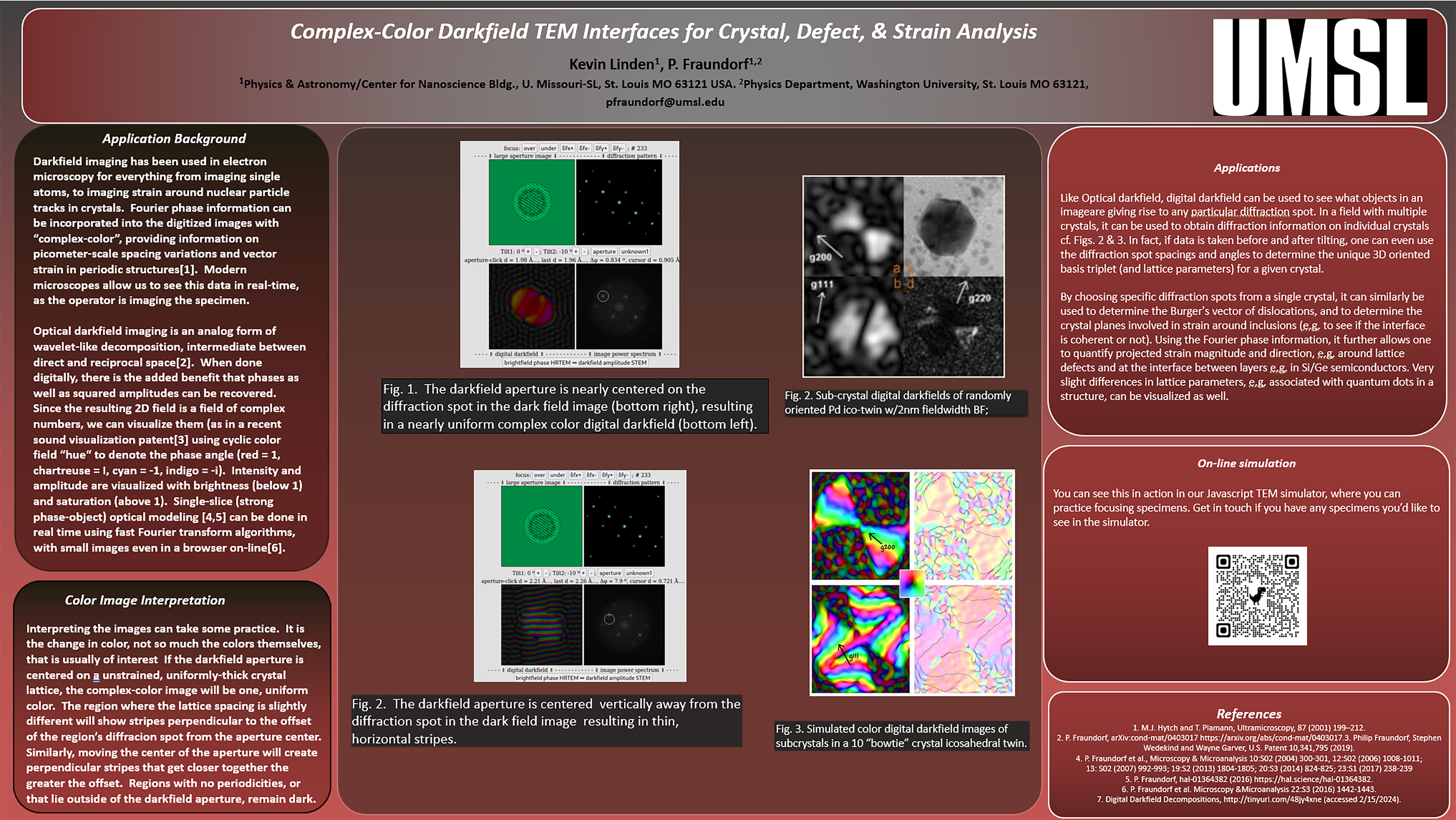
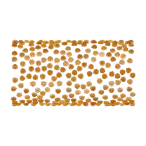
Optical darkfield imaging in microscopy involves forming images of a specimen (below left) using a back focal-plane (scattering angle) aperture that excludes the unscattered beam. It's called "dark field" because the field surrounding the specimen doesn't scatter, so it's dark. The digital darkfield animation below illustrates this by placing an aperture (centered in the orange figure below) over the power spectrum (a digital substitute for the back focal-plane's optical diffraction pattern) here shown with the DC peak (or unscattered beam) below center. In this example, only nanocystals with projected periodicities that diffract into the aperture light up in the darkfield image at right, and this varies with aperture position. In this case, the aperture is moving by 1.25 degree increments around the ring associated with diffraction from gold 2.3 Ångstrom (111) lattice spacings. A larger traverse at 2.5 degree increments can be found here.

Below some ImageJ amplitude darkfields, of 2.3 Angstrom periodicity along various directions in a lattice image, combine with fringe visibility theory to analyze the crystallographic relationship between some nanoparticles and a cylindrical structure on which they lie.


Here's a snapshot from application of digital darkfield periodicity mapping techniques to columnar quasi-epitaxial growth of Cu2O on single crystal silicon, synthesized in Jay Switzer's lab at UM-R.

Here's a snapshot from the application of digital darkfield periodicity and strain mapping to hidden icosahedral twins, which we've for example seen in electro-active polymers developed by a company in the St. Louis area as well as in metal nanoparticles prepared by Max Bertino's group at UM-R.

Possible Related Materials
* In addition to outlining a quantitation process for considering multiple reflections from the same image, Martin's maps of three at-first-glance-invisible quantum dots in a HREM image (below left) detail a 9.0 picometer (0.09Å) increase in GaInP's d002 = 282.6 picometer (2.8Å) lattice spacing as one moves across alternating Ga0.52In0.48P and InP layers only ~2 nm (20Å) in width (below right). Fringe spacings found on the InP bands are typically within 1.9 picometers (0.019Å) of the expected values for pure InP relative to matrix, if we ignore averaging effects likely to bring theory even more closely into agreement with Martin's measurements. The contours show that this amounts to a local increase in fringe spacing from about 10.98 to 11.33 image pixels (each spanning ~25.0 picometers or ¼ Å), as one moves from the GaInP matrix into an InP quantum dot. This is precise work for digital interferometry on images whose point resolution is near 200 picometers (2Å), and only possible on images recorded in parallel (rather than with STEM) in the face of picoscale drift.
