The methods applied here are designed to work on experimental lattice images. This page illustrates their use instead on model lattices of a variety of interesting structures. For many of these, experimental HR-TEM images may be found elsewhere on our web pages. Notes on the techniques of calculation, with more examples, may be found here and here.
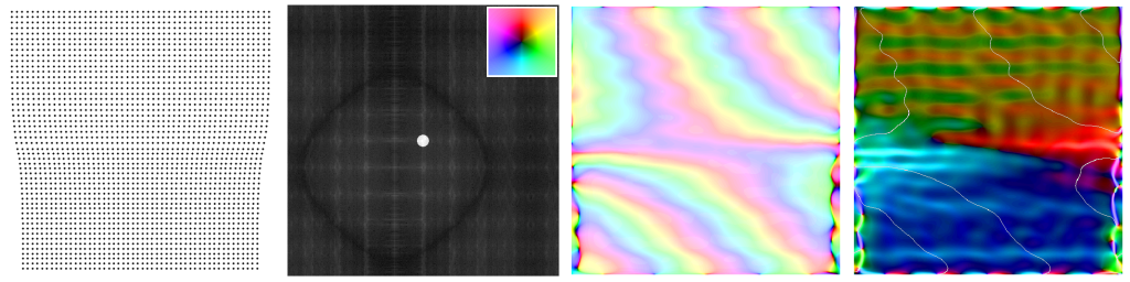
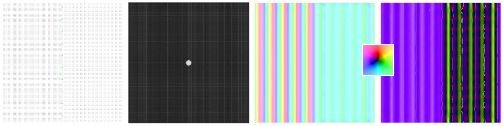
Panel Format (from Left to Right)...
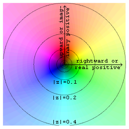
Below find a draft color key. For component color (where hue denotes direction in a 2D coordinate space and brightness denotes magnitude), the convention as one might expect is: rightward from center denotes increasing magnitude to the right, upward from center denotes increasing magnitude in the up direction, etc. For complex color (where hue denotes phase and brightness denotes amplitude): rightward from center denotes increasing real-positive amplitude, upward from center denotes increasing imaginary-positive amplitude, leftward from center denotes increasing real-negative amplitude, and downward from center denotes increasing imaginary-negative amplitude. The circle labeled |z|=0.1 in complex color (e.g. darkfield images) represents a complex amplitude of 1, but in component color (e.g. strain maps) it represents a magnitude of 0.1 for increased sensitivity at small values. Brightness goes up as magnitude or amplitude increases from 0 to this point, beyond which color saturation is increased instead.
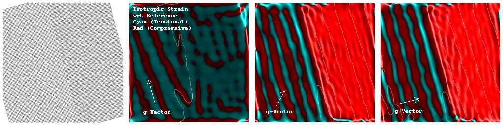
Note that the direction of the strain field (represented by component color in the 4th panel of each series) can also be inferred from the sequence of complex color bands in the 3rd panel. Thus for example a sequence of 3rd panel red-yellow-cyan-blue (RYCB) bands encountered while traveling along the direction of the g-vector (a vector in the 2nd panel from DC peak to the Fourier aperture) means a tensional strain, while red-blue-cyan-yellow (RBCY) in that same direction denotes a compressive strain. Many examples follow.
This exercise provides clues to the "line of no contrast", or butterfly shape,
taken on by isotropic inclusions in TEM 2-beam diffraction-contrast (and
especially darkfield) images. The line of no contrast is always perpendicular
to the g-vector or "operating reflection".
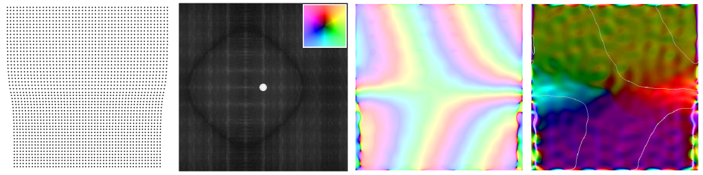
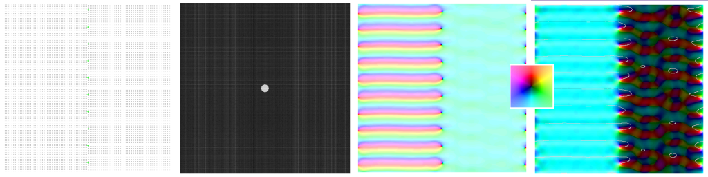
This more animated image shows what happens if we select different g-vectors (in the TEM: "operating reflections") in Fourier space for the calculation...
 In context of some earlier Mathematica notes on quantifying this model
(intermittently available on newton in Read More About It below),
it appears from above that regions of the specimen with strain
directions parallel to the g-vector (e.g. the yellow
inclusion in the 4th panel of the top image above)
are showing tensional strains relative to the reference
periodicity, while regions with strain directions antiparallel
to the g-vector (e.g. blue in that image) are compressed
relative to the reference. Thus as the operating reflection
changes direction (in the 2nd panel), so do the strain colors
of regions interior and exterior to the inclusion.
In context of some earlier Mathematica notes on quantifying this model
(intermittently available on newton in Read More About It below),
it appears from above that regions of the specimen with strain
directions parallel to the g-vector (e.g. the yellow
inclusion in the 4th panel of the top image above)
are showing tensional strains relative to the reference
periodicity, while regions with strain directions antiparallel
to the g-vector (e.g. blue in that image) are compressed
relative to the reference. Thus as the operating reflection
changes direction (in the 2nd panel), so do the strain colors
of regions interior and exterior to the inclusion.
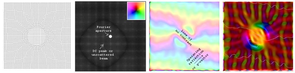
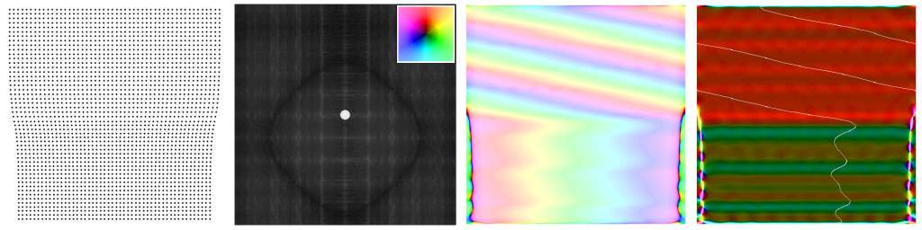
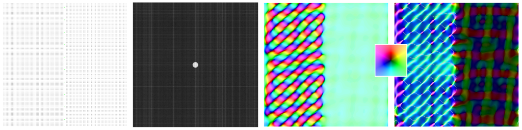
The above image may be moving too quickly for a close look. Below find one of those images standing still, with a number of features labeled. Note in particular the relationship between: fringe tilt/spacing as seen in panel-1, locations in the Fourier aperture of panel-2, and color-fringe sequences and spacing in panel-3. In experimental images where the panel-1 spacings or their variations are too small to see, the sequence of color-fringes in panel-3 will still provide a guide to what's going on.
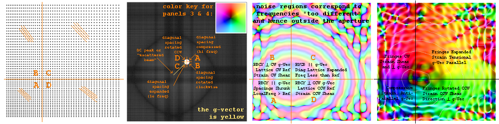
In particular, panel-3 color-fringes encountered while moving in the direction of the "g-vector" indicate spacing variations which are compressed (strained opposite to the g-vector direction) if the color-sequence is RBCY, and expanded (strained in the g-vector direction) if the color-sequence is RYCB. The size of the fringe spacings, relative to the reference periodicity, can be determined by inspection since the frequency difference is the reciprocal of the color-fringe period. In other words, if d is the reference periodicity in panel-1, and w is the parallel color fringe spacing in panel-3, then the local periodicity d' in panel-1 obeys |1/d' - 1/d|=1/w.
On the other hand, panel-3 fringe spacings encountered by running perpendicular to the "g-vector" indicate spacings identical to the reference which are slightly rotated clockwise or counterclockwise with respect it. In this "rotation moire" case, the RBCY sequence direction perpendicular to the g-vector in panel-3 reflects the type of shear (CW or CCW), while the period of color-fringes encountered while moving in that direction determines the amount of rotation (shear magnitude) with respect to the reference periodicity. In fact, if a color fringe spacing of w in panel-3 is encountered running perpendicular to the g-vector in panel-2 of reference frequency g = 1/d, then panel-1 spacing d fringes are locally rotated relative to that reference direction by the angle phi = ArcSin[d/w].
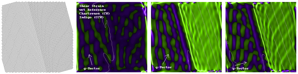
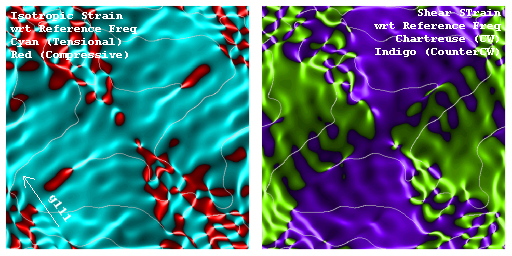
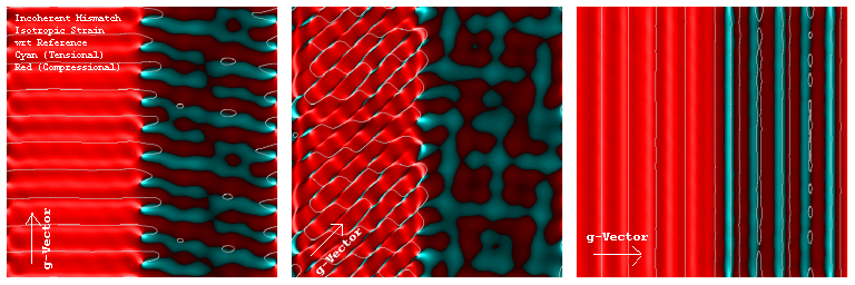
Another way to visualize the quantitative information in the panel-4 strain map is to break it down into a pair of bi-chromatic images representing components parallel and perpendicular to the operating reflection (or reference frequency vector). This is done in the figure below for the previous figure's gradient specimen strain map. The following sequence of orthogonal colors has been chosen for their mnemonic value: Strain parallel to the reference g-Vector (higher frequency, compressive) is represented by the hue 0.0 color red. Strain with a clockwise shear from the g-Vector has the hue 0.25 combination of yellow and green that might be called chartreuse. Strain anti-parallel to the g-Vector (lower frequency, tensional) has the hue 0.5 color cyan. Finally, strain with a counter-clockwise shear from the g-Vector is the hue 0.75 combination of blue and magenta that might be called indigo.
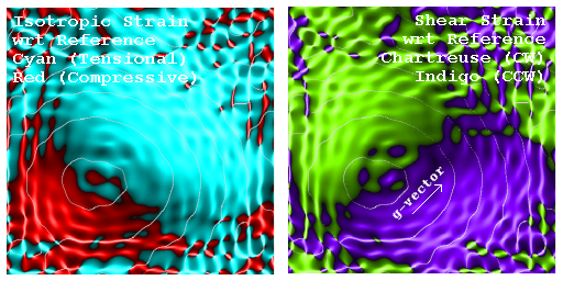
As a second example, the isotropic inclusion's component strain maps, from our first case study above, shows red compression zones at opposite ends of a line in the direction of the g-vector, regardless of the direction of the operating reflection.
If a field of view has more than one periodic object (e.g. crystal), that object responsible for a given spot in the power spectrum (or diffraction pattern) can be located by forming a darkfield image using that spot. Below find a simple image with two periodic objects lying on a thin, holey, amorphous film.
Also note in the above image that when the Fourier aperture used
to select the image is increased in size, more of the "shape transform"
of the periodicity is included in the image, yielding a higher
resolution view of the object in darkfield. Below, a second spot in
the power spectrum is used to highlight a different crystal in the
field of view.
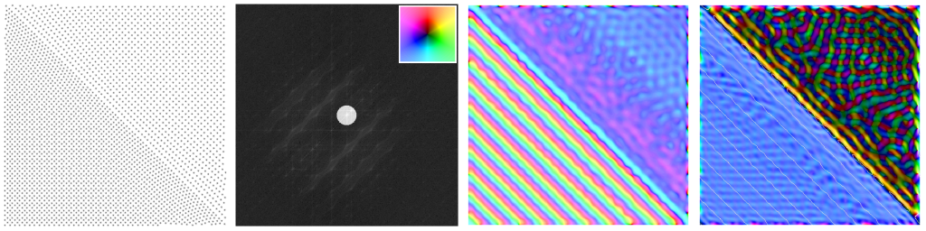
Many materials nucleate with icosahedral or dodecahedral symmetry on the atomic scale (e.g. to minimize surface area), but as they grow find that atoms away from the surfaces are better able to minimize their energy and disorder with a spatially periodic structure e.g. a face centered cubic lattice. Initially icosahedral or decahedral structures as they grow may then take on the shape of twinned structures. For fcc crystals like palladium, this often results in icosahedral twins comprised of 20 paired wedge-shaped crystals (one for each of the triangles on the surface of an icosahedron). If one "darkfield images" such a structure using one of the many diffraction spots seen when viewing it down an icosahedral 5-fold axis, the underlying crystal wedges show up in pairs. An example is this (002) bowtie...
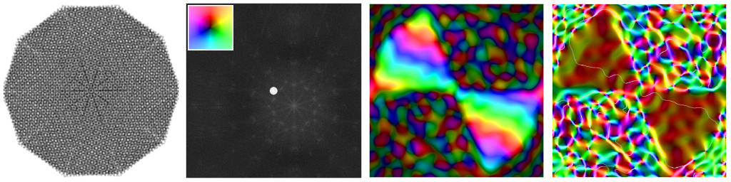
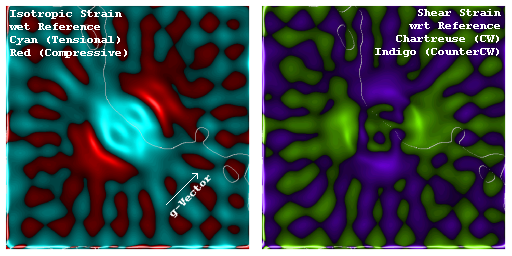
Another example is the (111) butterfly below, formed from two pairs of opposing crystals that share that set of planes and hence light up simultaneously.
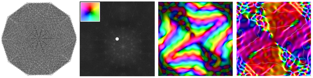
Of course, this conversion to fcc from icosahedral form is not done without objections from surface atoms. Note for example in the butterfly's strain image (4th panel) the tensional strain line (increasingly narrower bands in the g-vector sequence red-yellow-cyan-blue) running radially outward along the boundary between adjacent crystal pairs.
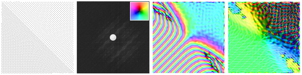
When the tensional displacement between fringes increases past half a lattice period, it begins to look "compressive" to our algorithms, as can be seen from the butterfly's isotropic strain map below. However, the shear map next to it shows clearly (in agreement with the panel-3 fringe pattern mentioned above) that the adjacent crystal lattices are indeed rotated apart.
Note: The dislocation at left is easiest to see by printing the image out and looking at a low angle for a row or rows of atoms that abruptly end. This exercise contains clues to the way the "g dot b = 0 for dislocation invisibility" works when making use of conventional TEM diffraction contrast to determine dislocation Burger's vectors (which for these simple-cubic lattice examples is horizontal in both cases). Of course, Burger's vector is the offset one encounters after following any otherwise "closed path" in the lattice that encircles the dislocation's core.
The animations move the g-vector or selected periodicity in sequence from g10 => g11 => g01 => g11 => repeat.
Begin with a "homemade" misfit dislocation between two slightly different simple-cubic lattices. Note how the dislocation disappears when and only when the g-vector (and Fourier displacement) is vertical and hence perpendicular to the dislocation's Burger's vector.
Next consider a classical edge dislocation in homogeneous material, created using equations from Hirsch et al. They say that the displacement parallel to the Burger's vector b (which in these examples is one lattice unit of horizontal offset) is R_b = (b/2pi)[Phi + Sin[2Phi]/(4(1-nu))], where nu is Poisson's ratio (a typical value might be 1/3), and Phi is an angle from dislocation line to the sample point which equals zero in the direction of -b. The displacement normal to the slip plane and perpendicular to b (which in the above dislocation model was set to zero) is R_n = (b/2pi)[((1-2nu)/(2(1-nu)))ln|r| + Cos[2Phi]/(4(1-nu))].
Again dislocation contrast in the strain map almost goes away when the g-vector is vertical.
Look for some fcc and dcc examples here next.../pf
Here is a case of 2D area-preserving epitaxy between a large lattice (on top) and a smaller lattice (at bottom). I say area-preserving (e.g. as distinct from volume preserving) because I've simply required that if a lattice parameter is stretched by factor f (greater than 1) horizontally (e.g. to line up with the lattice points above and below) that the orthogonal (here vertical) lattice spacing be compressed (divided by f) so as to keep the product of the two constant. I've also then added an e-folding scale distance for both lattices to relax back to their preferred values over a distance of about 5 cells.
Note that the "two color patch" effect we've seen in experimental images of Si/Si-Ge seems to pop up here. A similar effect (as in the experimental case as well) occurs in the diagonal reflection case. Hence although nothing here is quantitative yet, this is an encouraging proof of concept.
Start with a g-vector perpendicular to the plane of the epitaxy. Red in the top lattice (strain parallel to the g-vector) denotes an up-down tensional strain in comparison to the reference periodicity. The darker but still green color in the lower half of the strain image suggests that the reference spacing is nearer to, but not quite aligned with, that lattice's smaller periodicity.
The diagonal g-vector darkfield image and strain map below uses a reference not close to either the top or bottom lattices, and a new feature (the red/cyan contrast) begins to emerge along the interface.
Finally, imaging this system with a g-vector in the plane of the epitaxy shows lateral tension (yellow-green) in the top layer, lateral compression (blue-magenta) in the bottom layer, and an even more pronounced pair of alternating shears (red/cyan) along the interface. Note that in progressing rightward the shears go from cyan to red, while in the dislocation images above (in which the compressed lattice is also in the bottom half of the picture) the shears go instead from red to cyan. This is not surprising, since a periodic array of misfit dislocations can indeed be used to cancel out the buildup of strain at mismatched lattice interfaces.
To clarify what is happening, we next look at a larger region of the interface. This model has been tilted so that the interface is not parallel to the field edge, and projected potentials have been averaged over adjacent pixels to minimize moire effects. Also the reference frequencies have been adjusted to closely match the base frequencies in the larger of the two lattices.
We begin using a g-vector perpendicular to the interface plane. Note the dark absence of strain in the upper-right corner (where our large spacing reference cells are relaxed). Note that this gives way to a tensional strain (yellow), due to expansion of the cells in a direction perpendicular to their compression, as one approaches the interface. On the lower-left side of the interface, we see a compressional strain (blue) which begins a bit larger (brighter) and then levels out as one moves into the relaxed region of smaller unit cells. Note that the direction of the strain field can also be inferred from the color sequence of bands in the 3rd panel. Here a sequence of red-yellow-cyan-blue bands encountered in the direction of the g-vector means a tensional strain, while red-blue-cyan-yellow in that direction denotes a compressive strain.
The second plot uses a g-vector parallel to the interface plane. Note the compressional (green) nature of the strain in the smaller (lower-left) lattice away from the interface, as well as the alternating shears as the different lattice periodicities "beat" against one another along the interface. Could such alternating shears be responsible for periodic texture we've been seeing in experimental darkfield images, as one moves along unrelaxed lattice interfaces, or conversely does some sort of strain relief (e.g. slip, dislocations) simply have to be there? I suspect it's the latter, although a look at some even larger regions (where the strains away from the center point become ridiculous) will probably clarify.
Next step on modeling epitaxy: How about an array of misfit dislocations to relieve the strain? Before getting too fancy, consider a simple juxtaposition of lattices whose spacing ratio is 10/9. At the interface, which for variety runs vertical in these images, we've marked in green locations where atoms in the smaller lattice (left) line up halfway between atoms in the larger lattice on the right. The "half atom" locations occur every 10 of the smaller lattice points, or 9 of the larger lattice points.
When the g-vector is perpendicular to the interface (here to the right) and centered on the frequency of the larger lattice, one gets a compressional strain in the smaller lattice on the left, but not a lot of fine structure otherwise.
However, when the g-vector is parallel to the interface (here
directed upward), one gets an alternating pattern of shears centered
on the "half atoms" at the interface, in addition to a compressional
strain in the smaller lattice on the left. Note also that the
compressional strain bands in the 3rd panel, running perpendicular
to the interface, necessarily get disposed of as they approach
the interface -- the only question is precisely how they are made
to vanish (e.g. as shown below with no effect on the Si-Ge, or in
locally-compressed edge dislocations at the half-atom points
with regions of coherent lattice under tension in-between).
This 10-atom "misfit periodicity" persists when the g-vector is at 45 degrees to the interface (here to the upper right), suggesting that it may show up in lattice images of more than one set of lattice planes.
Examining isotropic strain only, for the various g-Vectors, shows that all fringes examined in the lattice on the left are indeed compressed relative to the right hand side reference. Also note the alternating blue/red spotting at the "half atom" points on the interface, in the first panel (g-Vector in the plane of the interface) and to some extent in the 45 degree fringe strain map as well. My guess is that, if the interface becomes coherent except for misfit dislocations at the half-atom points, these strains are then spread out across the gap between those points. The only other way to cash in on the energetic advantage of a coherent interface is to make the interface perfect, but then pay the volume-proportional price of having the top lattice stretched so as to follow the cadence of the lattice below.
A similar plot was done for shear strains, which alas seem to have various residual values away from the interface on the left hand side which I don't understand at this point, and might be a sampling artifact.
The foregoing may be considered an "incoherent extreme", just as the idea above of a coherent interface allowed on both sides to relax back to normal dimensions, laterally as well as in the growth direction, is a "coherent extreme". We now turn to a coherent strained model, but one in which lattice spacings lateral to the interface are fixed, while out-of-plane lattice spacings respond to complement the lateral strain at the interface, but then relax back to bulk values (e.g. with help from point defects) with an e-folding distance of about 15 units here. This model is suggested as useful by experimental strained-lattice work underway at present.
As you can see, there is little isotropic or shear strain to be found when the g-Vector lies in the plane of the interface. By comparison, however, the compression on the small unit cell (upper right) of the interface is clear with both diagonal and normal reflections.
The weak but unambiguous clockwise shear on the small-cell side of the interface I don't yet understand, and suspect it may be spurious (e.g. very sensitive to reference alignment).