Ring rotators and artificial gravity

Navigation bar: [intro] [puzzler] [explore] [discuss] [digress] [t'snext] [resources] [credits] "Go back" to return.

Put on your Sherlock Holmes hat and practice deciphering the whispers of nature provided by this model of a rotating ring with adjustable-radius. It's designed to give visitors a feel for (to even let them take data on) what happens as they change the radius of the spinning ring from its maximum allowed value (around 45 earth radii) to its minimum allowed value (the size of a good-sized virus molecule containing tens of thousands of atoms). It is also designed to be used by intro-physics teachers wanting to briefly extend the class discussion of circular motion toward its large size-scale (relativistic) and/or small size-scale (quantum-mechanical) limits. An incidental bonus is that it might give visitors a sense of changing physics on different size-scales as well.

Before we examine the limits, let's first consider loop-rotation at any speed. When you put your mouse over the figure below, the red lines and/or arrows pointing radially outward denote the local direction of the artifical gravity (and "fake" centrifugal force) that accelerated organisms riding on the ring might measure with a spring balance, and invoke to explain what happens e.g. when they try to jump "up" toward the center of the ring. From the map-frame perspective shown here, of the rotating ring's center of mass, of course objects riding the ring are being accelerated inward towards its center (centripetally) as they follow the circular path. Rather than going up and coming back down, for example, objects thrown "up" toward the ring's center simply follow a straight line path that eventually runs them into the ring further around the circle. The concept of artificial gravity nonetheless remains useful for organisms living on the ring, and is an example of a kind of geometric (or "affine-connection") force that Einstein's equivalence principle for general relativity has shown to be useful from all kinds of accelerated perspectives.

All such locally-useful geometric forces have two important features in common. First, they seem to act on every ounce of an object's being, e.g. like the apparent force when driving around a curve that pushes you toward the outside, and like the gravity on earth that keeps you from floating off into space. Secondly, there exists a locally-inertial frame of reference from whose perspective this force doesn't exist at all. In the case of the ring below, and for the case of the car taking a curve, one such locally-inertial frame is that of the stationary observer who is in fixed position with respect to the curved path. In the case of gravitation on earth, freefall frames (e.g. orbit and rain frames*) are locally inertial.

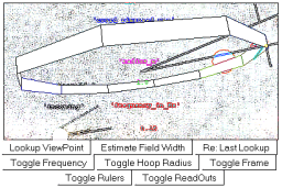
Slide your mouse cursor over the image below, and the ring should begin rotating with red lines and/or arrows denoting the direction of the "artificial-gravity". These vectors (originating from points on the ring) are equal in size and opposite in direction to the radially-inward centripetal acceleration that each part of the ring experiences on its path around the center. Instructions for changing your vantage pont and adjusting the ring radius may be found below. After playing with these a bit, try to adjust the radius for the loop until the artificial gravity is "one gee", i.e. 9.8 meters per second squared. Is this size reasonable? Any thoughts on how it might allow you to design an interesting amusement park ride? Would a large hoop with "one gee" of artificial gravity (e.g. the size of a space station, an L5 space colony, a covenant halo, or Larry Niven's ringworld) require rotation frequencies smaller, or larger, than 0.16 Hertz?

(* to do: _ add projectiles whose size and type varies with radius _ add javascript buttons to hop to large and small size limits *) (* here a set of independent variables is initialized *) (* the Mathematica model update commands follow *)

If you've used the simulator above to successfully estimate the radius needed by a "1 radian per second" rotating hoop so that it generates "one gee" of artificial gravity, you might also consider taking some data on how the acceleration varies as a function of hoop radius, at this fixed angular frequency. Can you find a theory in the literature (or in textbooks) to compare your "experimental results" with?

A quite different question: What does "locally-useful" mean in a quantitative sense when applied to such geometric forces? For example, over what distance and time and velocity ranges does the idea of a radial artificial gravity force begin to yield errors of more than 5 percent in the predictions that it makes?

On the left, we've made an attempt at plotting upper (blue) and lower (red) limits on rotational frequency as a function of hoop radius. Try plotting some of the data you've taken with the simulator on this plot. Is the data you've taken consistent with what the plot predicts? The dashed line on the plot tracks rotational frequency for hoops that provide an "artificial gravity" for their riders of 1 "gee". For the upper limit, we simply needed the value for lightspeed c. At the low end, we also needed the value for Planck's constant h, and a mass distribution model for our hoop. Nominal masses are figured by setting hoop mass, per unit of length of perimeter, to 10[kg/m³]×r². In effect this sets the shape-density product ffρ of hoop fractional width, thickness, and density to 10[kg/m³]. This works e.g. for hoop width of 0.1 r, hoop thickness 0.01 r, and density 10[g/cc] and hence for solid macroscopic structures familiar on earth.

What equations would you use to generate this plot? More importantly, are the equations used here reasonable? If so, what does this plot mean for the rotation of solid hoops smaller than a picometer in radius? Such hoops are still a thousand times larger in radius than an atom's nucleus!

Proper-speeds over a foot per nanosecond

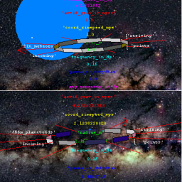
The lower half of the figure at right illustrates what happens when the hoop radius approaches its upper limit. The hoop radius is now much larger than the diameter of the blue-green planet shown in the background of the upper half image. To hold angular frequency at one radian per second, of course, the velocity of the rim also has to increase. The radius in the bottom-half image requires a rim velocity of one lightyear per traveler year (a coordinate-velocity of 0.707 times lightspeed). Note that at this speed, the segments of the hoop are no longer connected. Ropes running through the center (or perhaps some telescoping expansion joints) will be needed to hold the segments in place! This is one concrete way to visualize the effect called length contraction. Organisms riding the rim of course don't find themselves shrinking. Instead, to them the perimeter length as determined by a series of laser distance measurements around the rim** seems to be increasing beyond the value expected by multiplying the radius value by 2π. This happens in spite of the fact that their laser measurements of the radius show the same value as when the platform was not spinning. Thus to them spacetime seems no longer Euclidean.

Quantizing the loop's rotation period

If you reset the ring radius to nearer its lower limit (e.g. by clicking twice after startup on the Toggle Hoop Radius button), you can then pause the simulation and resize the radius incrementally toward its lower limit. The simulation only allows integral values for the last five quanta of angular momentum. This requirement arises (at least if we think of the rim as a bead following a circular wire) to ensure that the deBroglie phase of the bead (e.g. of wavelength h/momentum) obeys periodic boundary conditions around the loop. Does this condition also apply to a hoop rather than a bead, and are the radii allowed in the simulation consistent with what you expect for hoop radii values able to rotate at the specified rate? Conversely, could you use these observations to experimentally determine Planck's constant in the universe being simulated?

The plot at left illustrates the freeze-out process for ring rotators of typical matter density, on a kinetic energy versus momentum plot. The wave nature of the rotating ring is responsible for quantization, so at the minimum spin rate the circumference of the rotating ring is equal to one deBroglie wavelength. As you can see from the plot, rings with circumference much below 1 nm have spin cutoffs above room-temperature kT. This is consistent with the fact that polyatomic gas molecule rotation (for storing thermal energy and thus increasing heat capacity) may "freeze out" at sufficiently low terrestrial ambient temperatures. Local isocontours for the H₂ molecule's n=1 point are plotted by way of example. Note also that contours of constant speed have a unit slope (rise/run), while at low speed and fixed ffρ: contours of constant rotation frequency have a slope of 5/4, lines of constant mass and radius have a slope of 2, and lines of constant angular momentum (quantum number n) have a slope of 5. Would lines of constant centripetal acceleration (g-value) therefore have a slope of 8/7, and why or why not?

Here is a draft table of non-relativistic model numbers for a couple of diatomic molecules as well as for the ring rotators discussed above. It will not take into account relativistic effects for the large ring, as does the simulator above. It has other errors as well (don't be shy about pointing them out), so I'm inclined to consider this a placeholder only for the time being.

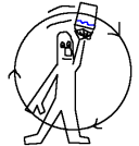
If you are up for a backyard test of these observations, try spinning a bucket filled with water in a vertical circle at arm's length. If you begin at high enough rotational frequency to keep the water from falling out of the bucket at the top of its arc, you can slow the rotation down until the water barely stays in. At that frequency the artificial gravity will equal 1 "gee". If it's a hot day outside, slowing down even further might cool you off. In any case, does what you find in this experiment agree with what the simulator above suggests will happen?

For those who'd like to flex their muscles as experimentalists on something other than rotation for a moment, consider measuring the flux (number per second) of incoming projectiles per unit area. How big is it, and is it the same in all directions? How does it vary with the size of the hoop? Also, at what distance do the projectiles cease to be visible? How does that vary with hoop and/or projectile size?

What's next for this page? More illustrations, more class exercises and puzzlers, more data, and more theory. To the applet itself we hope to add resizing buttons, buttons to change rotation frequency, and (already started) projectile and other environment objects of size appropriate to the current radius being examined. Thus you'll have to look out for incoming buckyballs, viruses, interstellar graphite onions, solid-fuel rocket-exhaust sapphires, micrometeorites, meteorites, asteroids, comets, planetoids, moons, planets and perhaps even a brown dwarf or two as well as the current collection of meteoroid-sized shooting stars as you examine rotating hoops across the range of allowed radii. Perhaps a nearby space shuttle, planet, or star will begin to manifest their presence as well.

• The fasTrak homepage
• Our page on candle dances, Pauli exclusion, and quantum spins.
• Notes on metric-smart approaches to teaching mechanics.
• Our map-based anyspeed motion table of contents.
• Writeups with references related to this include these notes on...
  • anyspeed modeling,
  • one-map two-clocks, and
  • anticipation.
• Our powers of ten explorer.
• A 2005 intro-chem nanoquest.
• Lists of some Live3D and Jmol models here.

This page is http://www.umsl.edu/~fraundor/nanowrld/newlive/spinning.html. Acknowledgement is due particularly to Martin Kraus for his robust Live3D applet. The galactic panorama is copyright Axel Mellinger, and is adapted here with permission, from his 300MB All-Sky Milky-Way. Thanks also to former grad student researcher Noom Pongkrapan for the simulator border. Although there are many contributors, the person responsible for errors is P. Fraundorf. This site is hosted by the Department of Physics and Astronomy at UM-StL. MindQuilts site page requests ~2000/day approaching a million per year. Requests for a "stat-counter linked subset of pages" since 4/7/2005: .