

28 Feb 2010: for Microscopy and Microanalysis 2010, Portland OR.
Zero-loss/deflection analysis
by P. Fraundorf, K. Pisane (WVU), E. Mandell (BGSU) and R. Collins
Outside of microscopy the relationship between energy lost, and momentum transferred, is a subject that has found considerable application over the past 2000 years. In electron microscopes, amazing types of detective work have been done for years with momentum transfer (esp. diffraction contrast), but only in recent times has it become possible to routinely obtain quantitative information on energy lost as well as momentum transfer.
One simple and robust way to put this type of information to use is to group image-pixels according to the fraction of detected electrons removed from the zero-loss peak versus the fraction of incident electrons scattered outside the objective aperture. These plots show new promise as a robust tool for quantitative analysis of intensities in transmission electron microscopes able to form energy-filtered images.
The first figure (top right) on this page shows a map on which anyone can plot experimental observations of specimen brightness I/Io in a brightfield transmitted electron image (x-axis), versus the fraction of detected electrons (y-axis) that did not lose appreciable energy (e.g. more than a few ppm).
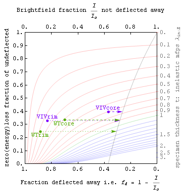
Lateral coherence effects aside, both of these are simple to understand experimental quantities between 0 and 1 for a given scattering experiment. Holes in the specimen by definition plot at the (1,1) point in the upper right corner, while regions too thick to permit electrons through plot at (0,0) in the lower left. An electron energy filter or spectrometer is needed to characterize the y-position of a specimen region on the plot, but not to obtain data on the x-position.
The colored contours on this first figure represent lines of constant thickness in units of the Egerton inelastic mean free path, i.e. for scattering inside a centered brightfield aperture. These contours assume a purely exponential (or range equation) model for both inelastic and angular scattering.
Exponential models do not work for coherent (Bragg scattering) from a single crystal. The tornado-like oscillating dashed line on the first figure illustrates this, by showing how one might expect single-crystal thickness fringes from a wedge-shaped specimen to oscillate contrast leftward from the curved light-black vertical exponential-model contrast-line on its right.
The idea of exponential mean-free-path is predicated on the assumption that scattering events remove particles from the unscattered set irreversibly, and dynamical single-crystal diffraction contrast illustrates graphically that this does not apply there since those oscillations come from electrons moving back and forth from the scattered to the unscattered beam. Diffuse elastic scattering, e.g. from individual atoms, of course follows the exponential model much more closely and so we may think of scattering in general as a process which has (i) orientation-independent exponential components, and (ii) more complex (and possibly-reversible) coherent-scattering components. Shifts to the left on the plot above may thus be seen as due either to incoherent scattering, or to something more complex that we might call "Bragg storage" since electrons in these orientation-specific states undergo near-parallel scattering processes just outside the range of brightfield-aperture detectability.
The brightfield zero-loss/deflection plots discussed above therefore allow one to quantitatively track momentum transfer processes (horizontal axis) detectable in electron microscope images, and energy transfer processes as well if one has a way to form energy-filtered "zero-loss" images.
Since inelastic scattering processes often reflect the number of protons per unit area between you and the electron source, zero-loss/deflection maps like that above can provide information on both the mass distribution and the "Bragg storage" associated with each pixel in a given bright-field image pair. If a hole region is available in the image, absolute values for the map fractions associated with each pixel may be obtained as well.
This type of measurement can be used to relate microscopic observations e.g. of nanoparticles in a field of view to macroscopic measures like the mass of a sample. For instance, the number of noble metal catalyst particles on activated charcoal supports per gram of sample may be of practical importance to many chemical manufacturing applications.
Zero-loss/deflection maps can also be used for quantitative comparisons of phase density, independent of phase crystallinity. One such application is determination of the density ratio between unlayered and layered graphene, in the core and rim of presolar graphite onions. Such ratio-determinations are illustrated in the second figure here, and discussed in the MSA paper above and in the references below.
What else might such zl/defl maps be useful for in the days ahead?