 .
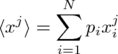
. The jth moment of random variable xi which occurs with probability pi might be defined as the expected or mean value of x to the jth power, i.e. :
.
The mean value of x is thus the first moment of its distribution, while the fact that the probability distribution is normalized means that the zeroth moment is always 1.
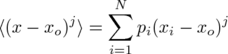
The jth central moment about xo, in turn, may be defined as the expectation value of the quantity x minus xo, this quantity to the jth power, i.e.
 .
.
The variance of x is thus the second central moment of the probability distribution when xo is the mean value or first moment. The first central moment is zero when defined with reference to the mean, so that centered moments may in effect be used to "correct" for a non-zero mean.
Since "root mean square" standard deviation σ is the square root of the variance, it's also considered a "second moment" quantity. The third and fourth central moments with respect to the mean are called "skewness" and "kurtosis", respectively. Note: Central moments are sometimes defined with an arbitrary center, instead of only the distribution mean.
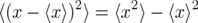
Playing with the above equations enables one to express central moments as polynomials in the uncentered moments. For instance, can you show that variance is the average of x-squared minus the average of x, squared?
Note: You may need to use the fact that the individual probabilities are guaranteed to add up to one.
More generally, I'm thinking one might say that:
 .
.
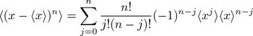
Even more generally, now using the binomial symbol in place of the factorial ratio giving ways to "from n choose j", one can show that central moments with respect to x1 and with respect to xo are related by:
 .
.
Examples to explore in this regard might include continuous distributions like the Gaussian (sum of probabilities for specific x-values gets replaced with an integral over all x), as well as discrete distributions like the Poisson.
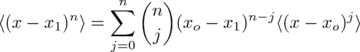
For instance the figure below plots the probability of k serious injuries in a bar fight THIS COMING FRIDAY NIGHT, for k between 0 and 20, if on comparable Friday nights an average of 2.5 injuries occur. As you can see, there is an 8% chance that nobody will get hurt, and a 20% chance that only one person will sustain injury. The figure also lists the zeroth through 5th uncentered moments, and the corresponding central moments (with reference to the mean).
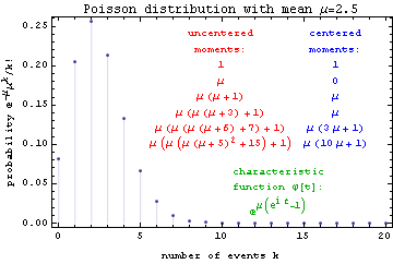
A similar plot for the continuous normal distribution with the same mean and standard deviation is provided below, for comparison. Note that in addition to being continuous (a feature that complicates the discussion of units with some surprisal based information measures), it also (unlike the Poisson) guarantees non-zero probability for negative values.
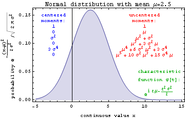
If all of the moments are in hand, one can in principle determine the probability distribution itself. One path to this result involves the distribution's characteristic function, which can be expressed by Taylor series expansion of the exponential thus yielding an infinite sum of moments:
 .
.
In turn, the jth moment may be recovered from the characteristic function by taking its jth derivative with respect to t followed by the limit as t goes to zero, and then multiplying by (-i)j. Caution: In the equations of this section only, i is the square root of minus one.
The figure above lists the first few moments, as well as the characteristic function, for the discrete Poisson distribution by way of example. Thus the moments give us the characteristic function of the probability distribution. Can we use this characteristic function to determine the probabilities themselves?
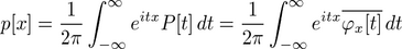
One possibility is to note that, using the "classical physics" convention for defining Fourier transforms, the characteristic function is the complex conjugate of P[t], the continuous Fourier transform of p[x]. Inverse transforming, and denoting complex conjugation or Fourier phase reversal with an overbar, we might therefore say that:
 .
.
Thus the characteristic function is little more than the probability distribution's Fourier transform.
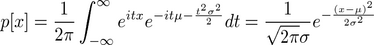
By way of example, consider the characteristic function for the univariate normal distribution given in the normal distribution figure above. The Fourier transform of its complex conjugate is none other than the univariate normal distribution itself, i.e.
 .
.
If only discrete values of x are allowed, per the summation notation above, the result should therefore be a sum of Dirac delta functions that are only non-zero at those values. Can you show this to be true for the Poisson distribution? By combining the first two expressions in this section, can we come up with a more direct expression for p[x] in terms of the moments? Does the result have convergence problems? Does it also bear a relationship to the expression below?
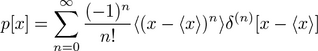
An interesting but perhaps more abstract expansion of probabilities, in terms of the central moments, is discussed in the 1981 American Journal of Physics article by Daniel Gillespie (AJP 49, 552-555):
 ,
,
where the delta symbol with (n) in the superscript refers to the nth derivative of the Dirac delta function with respect to its argument (in square brackets).
Although the above expression appears to be quite explicit, turning it into an explicit formula for p as a function of x can be non-trivial since derivatives of the delta function are normally defined by what happens when one integrates them over x. Hence some examples of this, in action, could help out a lot.
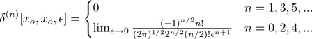
Gillespie takes this discussion further by noting that one can approximate derivatives of the delta function via the Gaussian distribution as a limit. This takes him to the odd assertion here:
 ,
,
wherefrom an explicit formula for probability at any point x in terms of central moments about xo may be obtained.
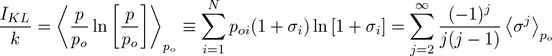
KL-divergence involves the comparing of two probability distributions, one (p) that we'll call actual and another (po) that we'll here call ambient or reference. Nonetheless KL divergence also can be written as an infinite sum of moments (or averaged powers), in this case of the dimensionless deviation from ambient σi=(pi/poi-1) for those two distributions. In other words:
 .
.
Here the subscript p on the angle brackets denotes an average over the actual (pi) rather than the ambient (poi) probabilities. Note also that use of the natural log rather than log to the base 2 yields information units of nats rather than bits. Low-order moments tend to dominate the infinite sum on the right, as long as σi=pi/poi-1<1 for all values of i. KL divergence converges even more rapidly in moments of σ averaged over ambient probability po:
 .
.
This latter equality uses the fact that the ambient average of σ is zero, and shows that for σ values much less than 1 that KL-divergence is approximately half the ambient probability estimate of variance σ2.
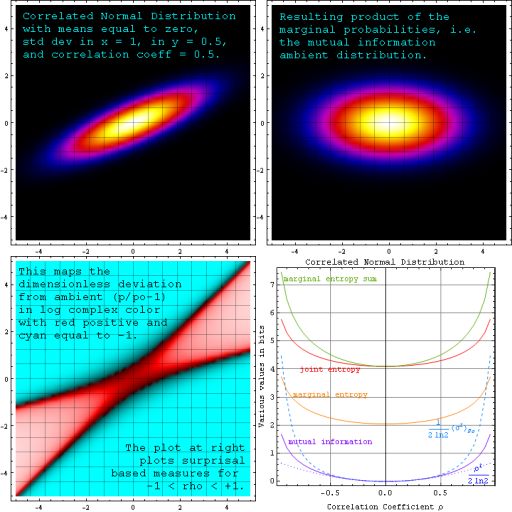
The figure below depicts a single bivariate (two-layer) distribution. Instead of comparing this distribution to an adhoc reference, we compare it to its own "product of marginals". In this way we can also compare mutual information as a measure of correlation, with the second-moment correlation coefficient rho that defines the distribution.
Along with depicting a correlated distribution spread across separate "layers" and the mutual information ambient that results, the figure also illustrates variation in the "dimensionless deviation from ambient" discussed above, and how various surprisal-based distribution measures depend on correlation coefficient ρ.
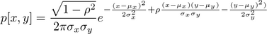
The bivariate normal distribution, from which the foregoing follows, can be written as:
 .
.
Note that the the subscripted sigma values in this equation represent standard deviations in x and y only for the uncorrelated case.
The distribution reduces to a product of two univariate normal distributions when the correlation coefficient ρ goes to zero, and to a 2D linear delta function along the correlation line as ρ2 goes to 1. As you can see, the mutual information associated with this joint distribution (i.e. the KL divergence with respect to the marginal probability product) is a measure of correlation that equals half of the 2nd moment of dimensionless deviation from ambient when ρ is small.
In the bivariate normal case, for small correlation coefficient, the plot above shows that mutual information in nats also goes as ρ2 over 2. Does a similar relationship between mutual information and correlation coefficient exist for other distributions as well? Regardless, mutual information and KL divergence are thus augmented versions of the familiar r-squared correlation-coefficient, designed to consider data on all moments of the probability distributions at work.
For more examples of this type of analysis, see our page on image multilayers.