Consider a 2 dimensional image with n pixels on a side, like the bivariate normal footprint in the last section on this moments and probability page. If each pixel were a positive number pij where i and j run from 1 to n, then by normalizing those arrays by the sum of all pixels one might look at moments as well as correlations between the x and y "layers".
If each pixel were instead represented by three positive floating point numbers, one each for its red, green and blue channel, then we might explore correlations between three pairs of six layers in a single color image. The number of states in each layer, of course, would be limited by the number of pixels on a side. Also note that in a 2D image, the layers would naturally occur in x,y pairs.
Look for more here, as this subject develops further. The good news is that any color image should be fair game for this analysis. As with life, pictures are more than mathematically representable objects since they can plug into innate human pattern recognition skills that go well beyond those that mathematicians normally consider...
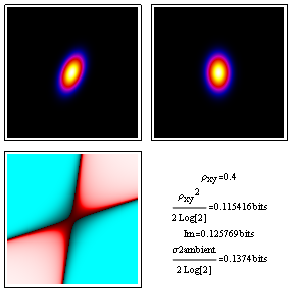
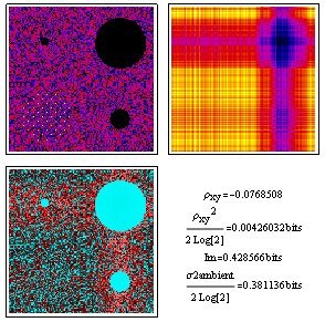
To make contact with our notes on moments and probability, here we've generated discrete bivariate normal distribution plot in image form for analysis. As you can see, the correlation coefficient squared relates nicely to the mutual information in bits. These approximations get better as the correlation coefficient's absolute values gets closer to zero.
A few notes about image locations and color tables are in order. The two probability distributions at top, namely joint on the left and the mutual information reference ambient on the right, are inherently normalized but displayed with ColorFunctionScaling active so that we get good blacks and good whites as well as a range of intermediate colors. The dimensionless deviation from ambient on the lower left, on the other hand, is displayed in logarithmic complex color (red is +1 and cyan is -1) with ColorFunctionScaling turned off so that each pixel contains quantitative information.
Similar display conventions are applied in the sections below, as well.
Perhaps the most familiar example of correlation measurement is that involving the r and r-squared correlation coefficients of a linear least squares fit. For data in a case like this with measurement errors in both x and y, our analysis above gives something like the following, where r is represented by rho_xy:
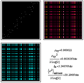
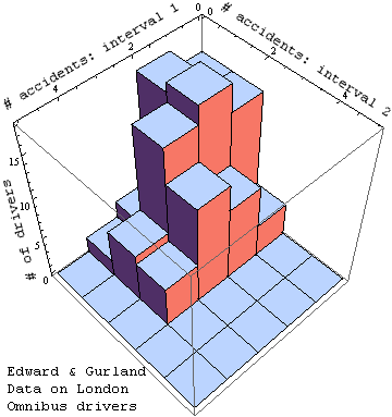
Correlated Poisson distributions (inherently discrete) are a bit messier to calculate[1]. The example below uses negative binomial marginal probabilities to generate a highly correlated distribution with a mean of 5.7 in the vertical direction and 9.6 in the horizontal direction. It might be used for example to model traffic accident data for a collection of drivers, like that for London Omnibus drivers shown at the bottom of this page.
In the figure here, the lower mean in the vertical direction might indicate that during the vertical-axis time interval the roads were much safer. The strong correlation might mean that something about a subset of the drivers nonetheless involved them in the lion's share of the accidents during the time periods on both axes. The mutual information reference ambient (top right) shows what the distribution would look like if the accidents happened regardless of who was driving.
As in the normal distribution case above both the correlation-coefficient estimate, and the dimensionless-deviation from ambient estimate, for mutual information become more accurate as the amount of correlation decreases.
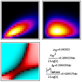
The experimental image below, taken with our EM430ST of a TiMn "quasicrystal approximate" with local 10-fold symmetry for Lyle Levine's dissertation over at Washington University, is clearly another story. The second moment correlation term is miniscule, but the mutual information term tells us nonetheless that variations in the x-direction clearly contain clues about variations along y. They just don't lie in the second moment terms.
This projected potential model reinforces the message of the previous image. Note that the variance in dimensionless deviation from ambient remains in the ballpark, even though the correlation coefficient is nowhere near the mutual information shared by x and y.
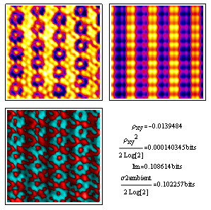
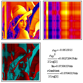
I include this because it's a classic standard for analysis by image processing algorithms, and unlike the two images above does not have much interesting going on in the Fourier transform (i.e. very few strong periodicities). Once more, xy correlation coefficient estimates fall short of the other two comparable measures, but in this case by less.
You'll also note that correlation analysis of the probabilities contained in these images, although it does provide information relevant e.g. to non-lossy compression of these images, does not include all information that x-variations might suggest about y-variations based on our experience in looking at other photos.
Thus for example if we saw two identical features in a horizontal scan, we might guess that they are eyes a corresponding vertical distance below which a nose might be found. Although this assumption might be correct in this case, you may not want to train the mathematics to expect this if one were instead looking at TEM specimen images like those above. Use of an ambient other than the mutual information ambient in KL divergence calculations, on the other hand, allows one to do just that i.e. to highlight correlations in the face of altered expectations.
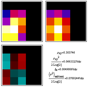
The next step here is to come up with some models for real niche networks which can be usefully displayed in the 2D format shown here. Although we are not there yet, to whet your whistle you might enjoy a look at this data on traffic accidents by 166 of London's Omnibus drivers, during two separate time intervals. Will the correlation coefficient provide clues to what accidents in the first time interval tell us about accidents in the second, or might we want to look at mutual information as well?
A breakdown of this data following the pattern above looks as follows:
More soon...
Footnotes