
This is a page about introducing unidirectional motion from a traveler perspective that works regardless of speed. It is powered by the 20th century discovery that time is a local variable, and that it is linked to a traveler's position through a space-time version of Pythagoras' theorem i.e. the local metric equation. The fact that time is local to the clock that's measuring it means that we can address the question of extended-simultaneity only as needed (with suitable caution) after the fact.

If we use this insight to describe motion with local traveler-centered (i.e. proper) variables, before the move to map-centered ones, good old three-vector velocities (proportional to momentum) and frame-invariant accelerations (albeit with frame-variant rates of momentum-change) become useful (especially for engineering problems) not only at high speeds but also in curved space-times (like that here on earth).
The focus here is not on fancy applications for these tools, but rather on introducing the concept of local time, and some of its applications, to introductory students in both high school and college physics courses when kinematics is first discussed. For the lion's share of students that are touched by physics courses, this might provide their physical intuition with a more solid conceptual-foundation from day one, even if the class moves immediately to a focus on applications of the Galilean-kinematic approximation.
This page on "metric-first kinematics" is only a stub at present. It is also complementary to a mobile-device ready site hosted by google. Please be patient as we work to develop them into a useful resource for teachers downstream.
To whet your whistle you might enjoy the summary below of a possible writeup, and the discussion of related student exercises below that. At the bottom you'll also find some more technical notes, for which some background in 4-vector analysis may come in handy. Extensive notes on use of this strategy with intro-physics classes are already available on the campus wiki for those with a campus ID.
Update: This working draft reflects downstream changes as we try to fashion a writeup for wide-accessibility e.g. in a journal like The Physics Teacher. Suggestions invited to that end.
 he world is full of motion, but describing it (that's what kinematics does) requires two perspectives:
(i) the perspective of that which is moving e.g. "the traveler", and (ii) the reference or bookkeeper
perspective which ain't moving e.g. "the map". Thus at
bare minimum we imagine a map-frame, defined by a coordinate-system of yardsticks say measuring map-position x with
synchronized-clocks fixed to those yardsticks measuring map-time t, plus a traveler carrying her
own clock that measures traveler (or proper) time τ. A definition of extended-simultaneity (i.e. not local to
the traveler and her environs), where needed for problems addressed by this approach, is provided by that synchronized
array of map-clocks.
he world is full of motion, but describing it (that's what kinematics does) requires two perspectives:
(i) the perspective of that which is moving e.g. "the traveler", and (ii) the reference or bookkeeper
perspective which ain't moving e.g. "the map". Thus at
bare minimum we imagine a map-frame, defined by a coordinate-system of yardsticks say measuring map-position x with
synchronized-clocks fixed to those yardsticks measuring map-time t, plus a traveler carrying her
own clock that measures traveler (or proper) time τ. A definition of extended-simultaneity (i.e. not local to
the traveler and her environs), where needed for problems addressed by this approach, is provided by that synchronized
array of map-clocks.
We will assume that map-clocks on earth can be synchronized (ignoring the fact that time's rate of passage increases with altitude), but let's initially treat traveler-time τ as a local quantity that may or may not agree with map-time t. The space-time version of Pythagoras' theorem says that in flat space-time, with lightspeed constant c, the Lorentz-factor or "speed of map-time" is γ ≡ dt/dτ = Sqrt[1+(dx/dτ)2/c2]. This indicates that for many engineering problems on earth (except e.g. for GPS and relativistic-accelerator engineering) we can ignore clock differences, provided we imagine further that gravity arises not from variations in time's passage as a function of height (i.e. from kinematics) but from a dynamical force that acts on every ounce of an object's being. In that case we can treat time as global, and imagine that accelerations all look the same to observers who are not themselves being accelerated.
Before we take this leap, however, we might spend a paragraph describing kinematics in terms of variables that allow one to describe motion locally regardless of speed and/or space-time curvature. These variables are frame-invariant proper-time τ on traveler clocks, synchrony-free proper-velocity w ≡ dx/dτ defined in the map-frame, and the frame-invariant proper-acceleration α experienced by the traveler, which for unidirectional motion in flat space-time equals (1/γ)dw/dτ where dw/dτ is the bookkeeper-acceleration in proper-units as seen in the map frame. Acceleration from the traveler perspective where the causes of motion are felt is key, because as Galileo and Newton demonstrated in the 17th century, those causes of motion are intimately connected to this second-derivative of position as a function of time.
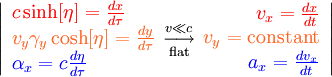
The relationships above allow us to write proper-acceleration as the proper-time derivative of hyperbolic velocity-angle or rapidity η, defined by setting c sinh[η] equal to proper-velocity w in the acceleration direction. These relationships in turn simplify at low speeds (as long as we can also treat space-time as flat) as shown at right below, because one can then approximate the proper-values for velocity and acceleration with coordinate-values v ≡ dx/dt and a ≡ dv/dt.

As mentioned above, treating space-time as flat requires that our map frame be seen as a free-float-frame (i.e. one experiencing no net forces). Much of the remainder of this course will therefore concentrate on drawing out uses for the kinematic equations on the right hand side above. We provide the ones on the left, to show that only a bit of added complication will allow one to work in curved-spacetimes and accelerated-frames where geometric-accelerations as well as force-related proper-accelerations have an impact on the bookkeeper-accelerations observed.
Scientific objectives: The objective here is to examine advantages of a metric-first approach to the description of motion, starting as early as a student's first introduction to unidirectional kinematics. Like the metric equation itself, the approach starts from the vantage point in flat spacetime of a single map-frame of yardsticks and synchronized clocks, but it explicitly recognizes that time-elapsed on a traveler's clock must be considered separately.
Results Overview: Proper (not coordinate) time/speed/acceleration underlie dynamics when coordinate-velocity v ≡ dx/dt = w/γ ≈ lightspeed c i.e. in both relativistic (w ≈ c) and hyper-relativistic (w >> c) domains. Proper-velocities (w ≡ dx/dτ = γv) add vectorially with help from an out-of-frame magnitude-only correction. Radar-time simultaneity allows one to explore space-time curvature using accelerated perspectives in flat space-time. All reduce to the familiar coordinate relations when v << c.
From the introductory physics student's point of view, to describe the motion of a traveler experiencing a uniform acceleration one might therefore begin by considering local-time τ on the clocks of that traveler moving with respect to local-time t on the synchronized-clocks of a reference map-frame used by everyone to measure position coordinate x.
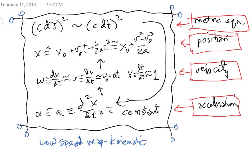
If one assumes traveler-time τ moves about as fast as local time t on the map-frame clocks, then as outlined above the motion of a traveler experiencing constant-acceleration (i.e. a persistent push from the traveler perspective) can be approximated by holding the second map-time derivative of map-coordinate x constant i.e. with motion described by parameters of the Galilean-kinematic (map-time t, coordinate-velocity v ≡ dx/dt, and coordinate-acceleration a ≡ dv/dt).
Of course, the flat-space metric equation says that the difference between these two locally-measured times can only be ignored at speeds low compared to the space/time constant (also known as "lightspeed") c.
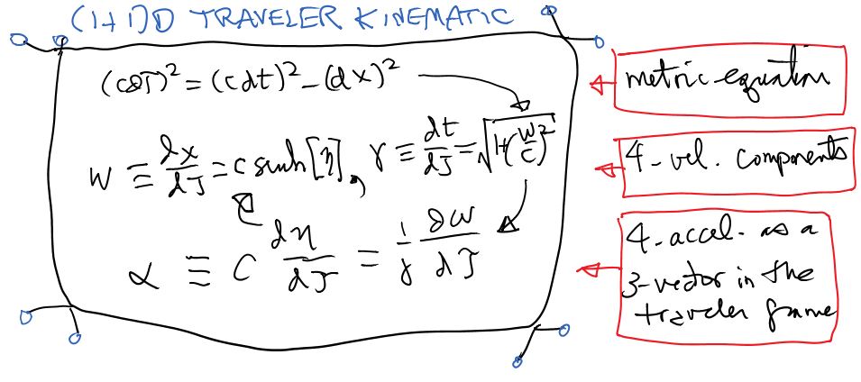
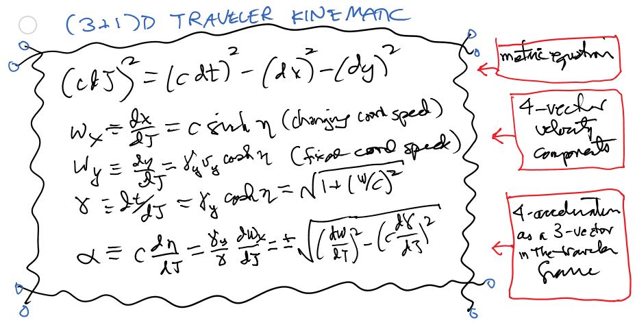
When differences between traveler-time τ and map-time t become significant, as outlined in the figure above, a traveler-kinematic (traveler-time τ, proper-velocity w ≡ dx/dτ, and proper-acceleration α = c dη/dτ) that works regardless of speed may be used instead. Thus Newtonian-kinematics is introduced from square one as approximation to a more robust approach that uses "frame-invariant" traveler-time as a local variable but otherwise operates in much the same way i.e. from the perspective of a single map-frame with (frame-smart addable) 3-vector velocities/momenta plus accelerated travelers of all sorts. As exemplified below, the approach extends nicely to motion in (3+1)D flat or even curved spacetimes, although our focus here is on the (1+1)D case.
In curved spacetimes, the distinction between bookkeeper-acceleration dw/dτ and proper-acceleration α becomes even more important. For example as shown in the figure below, "shell-frame" dwellers on a planetary surface must balance the inward geometric-acceleration GM/r2, associated with a stationary Lorentz-factor dt/dτ greater than one, with an upward proper-force capable of 1-gee acceleration, e.g. from a supporting surface, in order to prevent falling with the downward 1-gee bookkeeper-acceleration which is so dangerous for folks who make a career out of aerial acrobatics.

Aside: The Galilean-approximation to local traveler-kinematics, of course, also remains useful in accelerated-frames and curved-spacetimes with help from the equivalence principle, combined with geometric (affine-connection as distinct from proper) forces which apply mass-independent accelerations to every ounce of an object's being. We exploit this utility every time that we tell students to think of gravity as a downward force.

Introductory physics texts often start with: (i) time as an implicitly universal-variable, and (ii) the oddly mass-independent acceleration-due-to-gravity near earth's surface, as givens with no larger context. In this short note, we take an "engineering" rather than a "physics" approach and (for those who might enjoy it) invoke modern concepts to tell a story about: (a) time as a quantity like position that depends on one's choice of yardsticks & clocks, and (b) the geometric origins of gravitational acceleration. The note is designed to tantalize students interested in the subject with predictive equations within range of their math-background, while for students otherwise interested it provides context while delivering the good-news that their course involves only low-speed approximations.
This is space for class exercises that might be worth exploring. Suggestions invited. A complementary google-sites page is under development for other ways to network on this topic downstream.
It's nice to be able to derive detailed equations for constant traveler-acceleration for each of the model approaches discussed above. Nowadays, however, we can also go to computer programs for "second opinions" about the result. The trick in talking to computers, of course, is often in how to ask the question.
Two examples of such derivation setups, using Mathematica and starting from "instantaneous" differential relations, are now discussed in the draft of our companion paper. A third example for the (3+1)D case is linked here.
The differential relations themselves come from application of the metric equation (a differential relation itself) to the first and second proper-time derivatives of the traveler's position-time coordinate. The first derivative (regardless of the metric equation) yields a 4-vector velocity whose magnitude-squared is c2. The second-derivative yields a 4-vector acceleration whose magnitude-squared is the proper-acceleration α-squared.
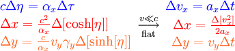
To be even more specific, the instantaneous differential variables in the (1+1)D traveler and Galilean cases are:
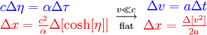
How might you ask a computer to integrate these, so as to write out the equations of unidirectional constant proper and coordinate acceleration something like this:
How about then adding a y (unaccelerated-component here in orange) term for a set of (3+1)D traveler differential relations, assuming that proper/coordinate-acceleration are only in the x-direction:
Here γy ≡ 1/Sqrt[1-(vy/c)2]. Are these results also consistent with the metric-equation constraints mentioned above?
Does integrating these simply add a y-component term (like that below) to the constant proper and coordinate acceleration equations for the (1+1)D case above?
The traveler-kinematic version at left may not be easily written in terms of arbitrary 3-vectors, because proper-acceleration α is a 3-vector defined in the traveler-frame while proper-velocities w ≡ dx/dτ = γv are 3-vectors for the traveler that live (as 3-vector momenta per unit mass) in the map-frame. Hence their various components don't add trivially, as velocity and acceleration components do in the Galilean case.
What other ways are there to ask these same questions to Mathematica, Maple, Wolfram Alpha, or other symbolic algebra programs? Also what other questions might one ask robot computers to chime in on in this same context?

That draft writeup introduces the space & time (then velocity & acceleration) variables used to track motion with help from Minkowski's space-time version of Pythagoras' theorem. The story is more complicated than the usual one because the distinction between time-elapsed on the traveler's clock (proper-time) τ, and time elapsed on synchronized map-clocks (coordinate-time) t, gives rise to proper and coordinate versions of velocity (w≡dx/dτ and v≡dx/dt) and acceleration (α and a) as well. Thankfully, all of these reduce at low speeds to the coordinate versions (t, v, and a) actually put to use in a typical intro-physics course.
An interesting model to illustrate these concepts at both low and high speeds is that of the "constant-acceleration" round-trip. A terrestrial-version of this roundtrip is illustrated in the animation at top right. Click on it for a discussion of some activities that might be fun to try with it.
The graphs to the right illustrate the quantitative predictions of Newton's equations for such round-trips, including the way that round-trip time for a given amount of acceleration is proportional to the square-root of the distance to be traveled one-way. Hopefully, clicking on that plot will provide clues to the underlying equations, as well as what happens when traveler-velocities (both coordinate and proper) begin to approach lightspeed c.

Time-dilation of course is not the subject-matter of an intro-physics course. However we argue that it's not a bad idea to provide examples early on nonetheless for two reasons: (i) It's cool; and (ii) The idea of specifying "which clocks" goes hand-in-hand with the idea of specifying "which yardsticks" i.e. your choice of coordinate-system.
This is therefore a sneaky but hopefully-fun way to deconstruct the notion of "universal time" otherwise implicit in some ancient worldviews (including Newton's). The figure at left is example of the kind of "local-time only" problem that students might enjoy thinking about, even if it is not going to help them on their intro-physics exams.
Although time-dilation across the breadth of an accelerated object is fun (and potentially confusing) to think about, we don't have tons of everyday applications to offer in this area. However, purely kinematic-acceleration as a source of space-time curvature in an accelerated-traveler's coordinate-system (particularly with help from radar-time definitions of simultaneity) is we feel an underutilized pedagogical tool since it can be addressed using only calculus and a few metric equations.

The four-vectors and four-tensors of general-relativity of course are needed to address the causes of mass-related space-time curvature, and allow for much simpler "coordinate-independent" expression of important relationships. When it comes to solving "boots on the ground" problems, however, the fact that students with much less math can start playing with these phenomena quantitatively is probably worth a closer look.
Although it may also be fun to think about your head aging faster than your feet, or the earth's surface aging faster than its center, the most oft-cited practical application of time-dilation associated with gravitational-acceleration is the gravitational-part of global-positioning-system time-dilation corrections. An earlier figure on this subject is posted for exploration at right, as well.
This older (2+1)D animation of a constant acceleration round-trip from map and traveler points of view uses co-moving free-float-frame simultaneity, as distinct from the more robust radar-time simultaneity used in the illustration of a single constant-acceleration leg below that.


A (1+1)D version of a single-segment acceleration using radar-time simultaneity from both map (left) and traveler (right) perspectives is shown here by way of comparison. Note that the curvy-nature of traveler coordinates in the x-ct diagram at left arises simply from accelerated-motion in the flat-space metric.

Question: Is there a metric-equation for acceleration-related time dilation as well as for the other two time-dilations mentioned in the writeup?
Possible answer: Yes. In fact these time relations all come from three expressions for what may be the same invariant-separation δs between events:
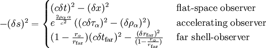
The first is of course the flat-space expression which may only work locally. The second is the local radar-metric in terms of coordinates τα and ρα measured by an observer undergoing constant proper-acceleration α in the +x direction (within the forward light-cone of acceleration's onset & the rearward light-cone of its stop). The third metric is of course the Schwarzschild metric mentioned, i.e. the metric at finite r from a massive object in terms of far coordinates. These metrics all offer different perspectives on ways to break down the same space-time interval δs into constituent time and space parts.
Note that technically, then, the "local zone" acceleration-related radar-time dilation might be more clearly written for a fixed lag-distance L as:

Here only the last and least-accurate approximation above for L << c2/α is the square-root of 1-2×energyratio (i.e. mαL/mc2) mentioned in the writeup. Nonetheless the form has mnemonic value for comparison to the other two types of dilation treated.