Algorithmic Complexity

Introduction

Algorithmic complexity is concerned about how fast or slow particular algorithm performs. We define complexity as a numerical function T(n) - time versus the input size n. We want to define time taken by an algorithm without depending on the implementation details. But you agree that T(n) does depend on the implementation! A given algorithm will take different amounts of time on the same inputs depending on such factors as: processor speed; instruction set, disk speed, brand of compiler and etc. The way around is to estimate efficiency of each algorithm asymptotically. We will measure time T(n) as the number of elementary "steps" (defined in any way), provided each such step takes constant time.

Let us consider two classical examples: addition of two integers. We will add two integers digit by digit (or bit by bit), and this will define a "step" in our computational model. Therefore, we say that addition of two n-bit integers takes n steps. Consequently, the total computational time is T(n) = c * n, where c is time taken by addition of two bits. On different computers, additon of two bits might take different time, say c₁ and c₂, thus the additon of two n-bit integers takes T(n) = c₁ * n and T(n) = c₂* n respectively. This shows that different machines result in different slopes, but time T(n) grows linearly as input size increases.

The process of abstracting away details and determining the rate of resource usage in terms of the input size is one of the fundamental ideas in computer science.

Asymptotic Notations

The goal of computational complexity is to classify algorithms according to their performances. We will represent the time function T(n) using the "big-O" notation to express an algorithm runtime complexity. For example, the following statement

Definition of "big Oh"

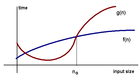
Intuitively, this means that function f(n) does not grow faster than g(n), or that function g(n) is an upper bound for f(n), for all sufficiently large n→∞

Here is a graphic representation of f(n) = O(g(n)) relation:

Examples:

• 1 = O(n)
• n = O(n²)
• log(n) = O(n)
• 2 n + 1 = O(n)

The "big-O" notation is not symmetric: n = O(n²) but n² ≠ O(n).

Exercise. Let us prove n² + 2 n + 1 = O(n²). We must find such c and n₀ that n ² + 2 n + 1 ≤ c*n². Let n₀=1, then for n ≥ 1

Constant Time: O(1)

An algorithm is said to run in constant time if it requires the same amount of time regardless of the input size. Examples:

• array: accessing any element
• fixed-size stack: push and pop methods
• fixed-size queue: enqueue and dequeue methods

Linear Time: O(n)

An algorithm is said to run in linear time if its time execution is directly proportional to the input size, i.e. time grows linearly as input size increases. Examples:

• array: linear search, traversing, find minimum
• ArrayList: contains method
• queue: contains method

Logarithmic Time: O(log n)

An algorithm is said to run in logarithmic time if its time execution is proportional to the logarithm of the input size. Example:

• binary search

Recall the "twenty questions" game - the task is to guess the value of a hidden number in an interval. Each time you make a guess, you are told whether your guess iss too high or too low. Twenty questions game imploies a strategy that uses your guess number to halve the interval size. This is an example of the general problem-solving method known as binary search:

Note, log(n) < n, when n→∞. Algorithms that run in O(log n) does not use the whole input.

Quadratic Time: O(n²)

An algorithm is said to run in quadratic time if its time execution is proportional to the square of the input size. Examples:

• bubble sort( notes ), selection sort, insertion sort