Molecule spatial harmonics
Visualizing reciprocal lattices ala diffraction

[pentacones] [equations] [cubic clusters] [sheets] [derivations] [puzzlers]
[pentacones] [equations] [cubic clusters] [sheets] [derivations] [puzzlers]
This note is for future "nano" crystallographers interested in structures which are both finite in size, and in part aperiodic. Emphasis is on the ability of electron diffraction to provide experimenters with real-time planar slices of a specimen's reciprocal lattice. Hidden beauty lies beneath those fuzzy patterns! To illustrate, we begin with an intricate small-molecule example considered in context of laboratory research here on carbon phases formed in red-giant atmospheres during the first half of this galaxy's lifetime. Some simpler classic examples (e.g. an fcc nanosphere, and a single graphene sheet) are provided below, along with some of the lovely equations* which make these calculations possible. Look for more on faceted and relaxed nanotubes/cones, as well as bamboo and herringbone nanofibers, soon.
Below find animation of a rotating 118-atom carbon pentacone on the left, and its diffraction pattern (or a slice through the center of its 3D reciprocal lattice) on the right. This is what one sees in an electron microscope diffraction pattern as the specimen is tilted under the beam. How good are you at "volume-visualization" from a rotating slice? To check this see what you can figure out about the 3D reciprocal lattice structure itself, which among other things includes for each of five faces: a straight "spike" that intersects the pattern center, three spike pairs that make it about half way into the center of the pattern, and another 3 pairs that make it only about 20% of the way in from the outer edge.

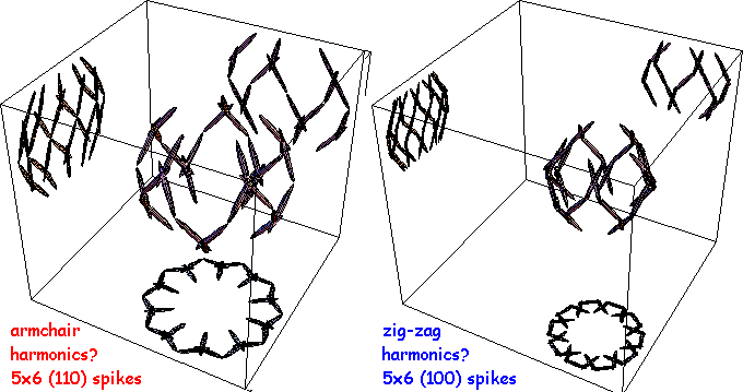
For example, the panel below superposes an inner circle associated with the spatial frequency of graphene's zig-zag rows (1/2.13A g100 reflection), and an outer circle associated with the spatial frequency of graphene's arm-chair or adjacent atom-pair rows (1/1.23A g110 reflection). There are 5 graphene sheets in this model, each of which has three g100 and g110 reflections. If you can identify 3x2 of these reflections in the course of a one-fifth revolution cycle, you will in effect have located all 30 reflections in the reciprocal lattice!
Because each of these reflections comes from an atom-thick sheet, in reciprocal space it will look more like pair of spikes (perpendicular to the sheet's plane) than a pair of spots. As these non-central spikes are rotated out of the animation's visualization plane (or the Ewald sphere in diffraction), their intersection with the plane shifts to larger radius. This foreshortening shift gives rise to "high frequency tails" on peaks in powder diffraction patterns of atom-thick crystals. Can you find evidence of this tailing to high frequency as the sheets rotate away from face on?
To get the ball rolling, note that the edge-on sheet which gives rise to the streaks in the pattern below is labeled on the left. Also labeled are the near-g110 "armchair" rows (in three of the five sheets) that give rise to those bright spots in lower left and upper right of the reciprocal lattice slice on the right.

Further clues to the nature of the 3D reciprocal lattice may divined from a look at the sequence below of x-y slices, moving down the z-rotation axis of the model above. Can you infer the location of the spikes in 3D from this animation, which runs through the sphere of g-values within 1 reciprocal Angstrom of the origin? Green intensities range linearly from 0 to 500 of Warren's single-electron scattering-intensity units. For fiducial purposes, the spherical shell at the spatial frequency of adjacent atom-pair rows (g110) is marked in red, while the spherical shell at the spatial frequency of zig-zag rows (g100) in graphene is marked in blue. For each of the five sheets, one spike is expected to run through the (000) peak which is white in the animation. Each sheet may also produce three pairs of spikes tangent to the red spherical shell, and another three pairs tangent to the blue spherical shell.

Yet another approach is volume visualization using a 3D contour plot or set of isosurfaces. The example below draws contours in x, y and z over the iso-intensity surface of value 500 in Warren's single-electron scattering units. From the top down, you can see the 10-fold projected symmetry. This particular plot covers g-values within a radius of 0.9 reciprocal Angstroms from the (000) DC peak (unscattered beam) in all three directions. Do you see any sign of the reciprocal space spikes discussed above?

With its staccato theme, the above figure suggests to me the harmonic analysis of a Bach melody, written for a universe with three time dimensions instead of only one! Click here for an interactive contour-plot of this reciprocal-lattice, which highlights it also as a potential source of design elements for Hollywood's next Klingon battlecruiser. Does being able to rotate and zoom this model in a variety of viewing directions help give you a better idea what's there, and perhaps to figure out what features of the original nanocone give rise to each? Interactive models of carbon pentacones in direct space may be found here, and ad-hoc models for zig-zag (100) and armchair (110) spikes may be found here and here.

Another question you might ask: How would the reciprocal lattice of a relaxed nanocone (shown on the right above) compare to that for the faceted nanocone considered here? Clues might be found in this animation, which shows green parallel slices through smaller 70-atom faceted and relaxed pentacone reciprocal-lattices, along with red/blue circles to help track g110/g100 sphere proximity as well. Intensity differences (e.g. faceted minus relaxed) for the 70-atom pentacone can also be visualized, in this case with annular reference-intensity shells set to 0 scattering-intensity units between g of 1 and 1.2, and to 100 units for g>1.2 reciprocal Angstroms. These differences are relevant, for example, to the analysis of powder diffraction profiles from single-walled nanocone assemblies.
Volume visualization techniques other than slicing and isosurfaces include direct volume rendering with diffuse-object scattering, and silhouette rendering via the Fourier projection slice (i.e. CAT scan's shadow-to-model calculation in reverse). For example, check out the 3D "shadow" below of the pentacone reciprocal-lattice, viewed from the same direction as that in the yellow-background "slice image" above. Note that the footprint of the entire reciprocal lattice differs significantly from that (in red) of the Ewald-intersecting slice. Imagine what the shadow will look like while rotating, then click on shadow-only or red-Ewald to see if those blobby reciprocal lattice spikes aren't now easy to identify.


The second cool equation which works for any molecule or crystal (even liquids and gases) is the Debye scattering equation below. It calculates the spherically-averaged powder-diffraction intensity profile Ipp as a function of scalar spatial-frequency g, in the same units. Note that these two equations involve only separations between atom pairs. Thus diffraction contains information about atom-atom correlations, but not e.g. about pair-pair correlations. Other tricks are needed (e.g. images) if one wishes to examine higher-order correlations.

If you are curious where these two equations come from, hang in there. You may actually like what you hear when we get around to it below**.
If you made it past the equations, you deserve a reward. Begin with the picture of a face-centered cubic (fcc) atom-cluster viewed down a <100> zone, but shadowed so as to show its projections down <110>, <111> and <112> directions as well. Can you figure out which of the shadows correspond to which viewing direction?

Now imagine a 34-atom spherical fcc nanoparticle, e.g. made out of Aluminum. Below find a 100-electron scattering unit iso-intensity plot for the body-centered cubic (bcc) reciprocal-lattice of this fcc nano-sphere. Note that the (000) spot (AKA the unscattered beam or DC peak) has been omitted by the contour plot routine in this case. An interactive direct-space lattice model can for comparison be found here, although it's up to you to check and see if it is fcc or bcc or something else. More about how changes in direct space structure affect reciprocal space structure may be found here. An illustration of how 2D diffraction patterns reveal this type of "crystalline" reciprocal lattice, as the specimen is tilted in an electron microscope, is provided here and at the bottom of this webpage.

For comparison to the fcc cluster case, and that of its reciprocal-lattice, projections of a small bcc cluster down <100>, <110>, <111> and <112> are shown below.

While we're at it, you might enjoy comparing the projections of the fcc cluster's reciprocal-lattice to that from a small diamond-fcc cluster as well. As you can see, this combination of projections and shadows makes cubic lattice symmetries fairly easy to identify, and of course also provides clues to their appearance in the electron microscope. For example, resolving the almost-overlapping spheres (dumbells) on the back wall is the challenge du jour for today's aberration-corrected TEM's.

Here is a preliminary calculation of the reciprocal lattice of a 114-atom hexagonal graphene sheet. This slice is taken with a view of the sheet face-on, but is the result so far of only a very low voxel-count calculation.

In three dimensions, this preliminary model shows three (100) and three (110) spike pairs perpendicular to the sheet plane, like the spike pairs expected perpendicular to each of the 5 pentacone facets above.


All of this connects to the world of the macroscopic crystallographer by going to the limit of an "infinite periodic crystal". There it is convenient to introduce unit-cell basis vectors a, b and c, and their reciprocal-lattice co-vectors a*, b* and c*. In terms of direct-space lattice parameters, the unit-cell volume is Vc = a . (b × c). From this the reciprocal-lattice (co-vector) basis is determined by the relationships...

If you made it past the derivations (bravo!), you may be ready for a puzzler. What reciprocal lattice is shown in green in this series of parallel slices? Hint: How many bright yellow dots does one encounter during the traverse? The red shell corresponds to the g110 (1/1.23A) spatial frequency of adjacent-atom rows, while the blue shell corresponds to the g100 (1/2.13A) spatial frequency of zig-zag rows, in a graphene sheet. Could you recognize it even if we sliced the same reciprocal-lattice in a random, rather than a symmetric, direction? What if we instead rotated a slice through the reciprocal-lattice center, as though it were the diffraction pattern of a molecule being tilted in the electron microscope?
