
Put on your Sherlock Holmes hat to analyze nano-structures here, using data obtained by real as well as simulated atomic-resolution imaging, diffraction, and spectroscopy. This page is inspired by the fact that when the number of atoms is small, these effects can be relatively easy to model. The focus, initially on models for prediction and pedagogy, is already shifting toward places to put YOUR experimental data (e.g. on lattice spacings and interplanar angles, or on characteristic x-ray peak intensities) into the analysis. In particular our lab produces individual 100-megabyte high-resolution TEM images that can serve, like a rosetta stone, as a source of clues for the decoding of messages written in structure from processes on the atomic scale. The first objective of this page is to provide our colleagues with tools to help them put electron-microscope hieroglyphics, from their own specimens, to good use.
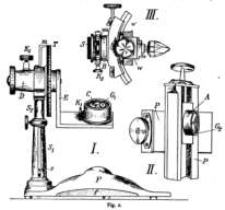
Note: The goniometer schematic in the upper left is a much reduced version of the drawing found in this early reference called to our attention by Peter Möck at Portland State University: "Über orientiertes Photographieren zum Krystallzeichnen" by V. Goldschmidt, Beiträge zur Krystallographie und Mineralogie (1919, Heidelberg) 1-6. Images of a modern-day goniometer for nano-microscopy may for example be found here. The images on the upper right are "experimental data" generated by an early version of the virtual goniometer made available on this page.To see how good you are already, try to identify the crystal structure of the default specimen loaded into the goniometer model below. What the heck is that stuff? Or at least, what are some candidate materials that it might be made of, based on the limited-accuracy diffraction and imaging data that the simulator can generate?
 When paused,
squares over the resizing points allow you to
"mouse drag" the crystal's lattice parameters in real time
to any values you like. The black
sliders below the table also allow you to manually
reorient the goniometer, which in effect acts like a tilt-rotate
stage when the side-entry tilt is near zero, and like
a double-tilt stage when the side-entry tilt is near 90 degrees.
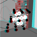
Hitting "s" with the applet selected toggles stereopair mode which
(with help from an image processing program like
ImageJ) can be
used to put together green-red stereopair illustrations
like that at right.
When paused,
squares over the resizing points allow you to
"mouse drag" the crystal's lattice parameters in real time
to any values you like. The black
sliders below the table also allow you to manually
reorient the goniometer, which in effect acts like a tilt-rotate
stage when the side-entry tilt is near zero, and like
a double-tilt stage when the side-entry tilt is near 90 degrees.
Hitting "s" with the applet selected toggles stereopair mode which
(with help from an image processing program like
ImageJ) can be
used to put together green-red stereopair illustrations
like that at right.
What follows is a list of practical analytical tasks, addressable with these developing tools, that we plan to illustrate with lattice images and/or diffraction data from past and ongoing nanodetective challenges.
The image below shows diffraction and HREM data from a polycrystalline grain found (thanks to the initiative of undergraduate researcher Nathaniel Hunton) in or on the unlayered graphene core of a presolar graphite onion. This onion and others were extracted by acid dissolution from the 1969 Murchison (Australia) meteorite by Roy Lewis and colleages at the University of Chicago, and ultra-microtomed by Tom Bernatowicz at Washington University. This slice was given the name "Jack" by former undergraduate researcher Dori Witt, perhaps because of the unusual non-circular bean shape which may be a result of collision between the diamond knife and the included grain. Only a limited number of crystalline phases have been previously identified in graphite onions like this, whose isotopes indicate that most of them were formed in the atmosphere of asymptotic giant branch stars (a major source of freshly-assembled carbon-atoms for the interstellar medium) during the first half of our galaxy's lifetime. Can the observed periodicities be explained by one of these previously identified phases?
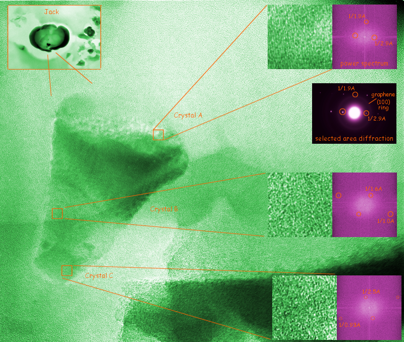
Many of the candidate crystal structures had no periodicities as large as the 2.9Å spacing, seen in both diffraction and high resolution imaging of the top half of the grain. One of the candidate phases which did, as pointed out by Kevin Croat at Washington U., is diamond face-centered cubic chromite (FeCr2O4) with lattice parameter a = 8.39Å. To check out the possibility, we clicked on the [New Space Group] button above until diamond face centered silicon was loaded into the goniometer. Clicking on [Download Model to Sheet Below] loaded silicon into the Crystal Structure and Orientation Worksheet. Changing the a, b and c values from silicon's 5.43Å to chromite's lattice parameter in effect loaded chromite into the worksheet. Pressing the [Update single crystal spot list below...] button then placed the 100 largest chromite d-spacings (with Miller indices between -6 and +6) into Table 1.
If the observed spot pair (2.9 Å, 1.9 Å, and interspot angle 90 degrees) has already been typed into the Indexer for measured spot pairs, one need only hit [Try to index...] to discover that no way to index with chromite exists for 2% spacing and 2 degree angle tolerances. However, adjusting the spacing tolerance to 3% shows that the pattern indexes beautifully with any of the 12 chromite <116> zones. The interspot angle is expected to be exactly 90 degrees if we can accept the first spacing as a chromite {220} with d = 2.97 Å and the second a chromite {331} with d = 1.93 Å. A closer look shows that no comparably visible spacings would be expected in such a pattern, so a possible indexing has been made. The 2.5 Å and 1.6 Å spacings seen on other crystallites might also be explained by chromite, although careful analysis of the 0.9-1.0 Å spacings and interspot angles would require a longer list of candidate spacings than is provided here at this time. EDS data showing Fe and Cr in the correct ratios might, for example, also be used to confirm such a proposed indexing.
Real soon now...
* Note that [uvw] is normally used to denote a specific (contravariant) lattice vector or crystallographic zone-axis, <uvw> a class of such directions or zones, (hkl) is the Miller index of a specific reciprocal-lattice point, covariant "g-vector", or set of crystallographic planes, and {hkl} denotes a class of symmetrically equivalent reciprocal-lattice points.
What's next here? More input/output and calculation options, illustrations, class exercises, puzzlers, data, and theory. We just added an ActiveWidgets spreadsheet to list g-vectors from a specific crystal. Only a few space-groups and simple crystal sizes/shapes are available now, but this will expand in days ahead, likely to include special structures like n-wall nanotubes and quasicrystal approximates, as well as arbitrary (even aperiodic) lists of atom positions. Tools (like SXTL) to match and index observed spacings and interfringe/spot angles may be next, along with buttons to record single-crystal/powder diffraction patterns and lattice images in 2D for closer examination. Eventually, we hope to offer, for example, independent variation of cluster size and shape, centering and extinction information lookup from any spacegroup (look for A, B and C centering soon, as it makes the single crystal indexing routine useful for any structure), Wycoff-format atom-coordinate entry tools, fringe-visibility maps, fringe probability/thickness plots, Kikuchi maps and other stereo-projections, strong-phase-object through-focus series, Cliff-Lorimer prediction of characteristic X-ray peak heights from elemental ratios and vice-versa, Debye-scattering profiles, formatted spiral powder overlays, some simple plasmon/dielectric and characteristic-edge energy calculations, select defect models including SPM topography and surface reconstruction predictions, and possibly even digital-darkfield analysis of images.
More importantly, tools for fitting data you've taken to specific candidate phases, and in some cases to directly-determined structural models, are planned as well. This experimental data might include observed fringe and diffraction spot spacings/angles taken at one or more specimen orientations, azimuthally-averaged diffraction/power-spectrum profiles, and eventually selected analyses of direct-space images. Data on widely-interesting phases will be programmed in locally, but we are also in discussion with developers and patent holders of searchable databases to facilitate more systematic comparison of data to known structures downstream.
On the nanoeducation side, empirical observation exercises with in-class peer-review are already under development here for a range of introductory science classes. The nano-goniometer above, when viewed from the side in "dual space" mode already offers an excellent interactive illustration of Ewald-sphere mediated diffraction. With sufficient refinement it is hoped that empirical-observation exercises like this, patterned on evolving real-world challenges, can work their way into classrooms, onto timed tests, and perhaps (if sufficiently robust) even into the larger culture of social competition and educational video-gaming. This page also provides possibilities to this end. For example, all crystals in the goniometer so far are in "c-axis" orientation, but a set of adjustable Euler angles will be added in days ahead to allow creation of "true unknowns" for analysis. What better challenge for prospective nano-detectives than to be given a device capable of performing quantitative experiments (of their choosing) on an unknown, and then showing how they can make the most of it?
As far as implementation is concerned, look for other applets (e.g. webMathematica, Jmol, and JavaView) to be put to use in the days ahead as well, and perhaps even a more interesting "room" in which to put the nanogoniometer. In all cases, we hope to make these tools available reliably and seamlessly (free where possible without the download of plugins) for use at many application levels, across the planet, in years ahead.
This page is
http://www.umsl.edu/~fraundor/nanowrld/newlive/crystal3.html.
Acknowledgement
is due particularly to Peter Möck at Portland State University for
his energy in exploring these matters, and
Martin Kraus
for his robust
Live3D
applet. Thanks also to Noom Pongkrapan for the
nano-goniometer border. Although there are many
contributors, the person responsible for errors is P. Fraundorf.
There are likely to be many.
Reports about bugs, ways to correct them, algorithms that might be
fun to implement, and interest/energy/time in helping out,
are most welcome via e-mail to "staff" at
newton.umsl.edu.
Putting "nanocluster" in the subject line might improve its
chances of getting through.
This site is hosted by the Department of Physics
and Astronomy at UM-StL.
MindQuilts
site page requests ~2000/day approaching a million per year.
Requests for
a "stat-counter linked subset of pages" since 4/7/2005:
.