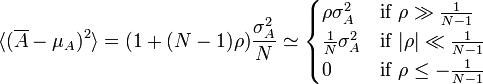
![\langle(\overline{A}-\mu_A)^2\rangle =\frac{1}{N^2}\sum_{i=1}^{N}\sum_{j=1}^N \sigma_{AA}[t_{ij}] = \frac{\sigma_{A}^2}{N} + \frac{1}{N^2} \sum_{i=1}^N \sum_{j\neq i}^N \sigma_{AA}[t_{ij}]](http://upload.wikimedia.org/math/9/4/8/948a923e3ad165b242b976f7398b82d3.png) ,
,An unbiased estimate of error in the estimate of a measured quantity A's "population mean" from N samples may be obtained by multiplying the standard error (square root of the quotient of sample variance over N-1) by the square root of (1+(N-1)ρ)/(1-ρ), where sample bias coefficient ρ is the average of the autocorrelation-coefficient ρAA value (a quantity between -1 and 1) for all sample point pairs. This is especially useful when values of A have been obtained from known locations in an n-dimensional parameter space x whose statistical properties are understood. In particular, when the sample is a three dimensional fragment of size D taken from a specimen of differing and randomly distributed but homogeneous grains of size d, sample bias ρ may be approximated by 1-(D/d)+(2/7)(D/d)2 when D≤d and by (d/D)3-(d/D)4+(2/7)(d/D)5 otherwise.
When microscopists make observations from a very tiny region but want to make assertions about the specimen as a whole, it's important to consider how representative that tiny sample is. Sample bias coefficient is a potentially robust second-moment statistical tool that may be directed to this end. The underlying theory, as well as some practical approximations, will be described and illustrated here in due time.
Using the defintion of autocovariance σAA[tij] for variable A sampled at points i and j on a manifold parameterized with the n-dimensional variable t, an unbiased estimate of squared error in the mean of variable A sampled at N known locations may be written* as:
,where the bar over A refers to the sample average which serves here as our unbiased estimate of population mean, and σA is the population standard deviation.
If we define sample bias coefficient ρ as the dimensionless average of A's auto-correlation over all sample point pairs, i.e. as
![\rho = \frac{1}{N(N-1)} \sum_{i=1}^N \sum_{j\neq i}^N \frac{\sigma_{AA}[t_{ij}]}{\sigma_A^2}](http://upload.wikimedia.org/math/c/4/a/c4a2f4a8e8a4cf6a1a6d99c31a4d2e0f.png) ,
,then this becomes
 .
.Thus sample bias coefficient relates uncertainty in the mean to the population standard deviation when sample bias, and not number of samples, is the main source of uncertainty.
If the population standard deviation is unknown and must be inferred from the sample, the uncertainties get worse. For that case, the above relation can be written in terms of sample variance sAA taken as a population, i.e.
 ,
,if we can show that an unbiased estimator for σA2 is:
 .
.That follows by expanding the definition of sA2 to show that:
 .
.As a result our unbiased estimate of error in the mean can written as:
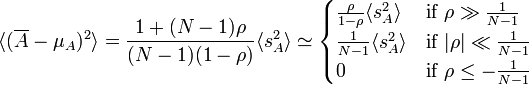 .
.A special case of this is the familiar expression for uncorrelated sample points, found in the center approximation above.
The plot below illustrates how the bias coefficient of a finite-sized sample can limit the accuracy of assertions about the specimen (or population) as a whole. Note also that a negative bias coefficient (when sample locations are anti-correlated) actually improves your accuracy, but that there are limits on how negative a bias coefficient can be for a large number of sample points.
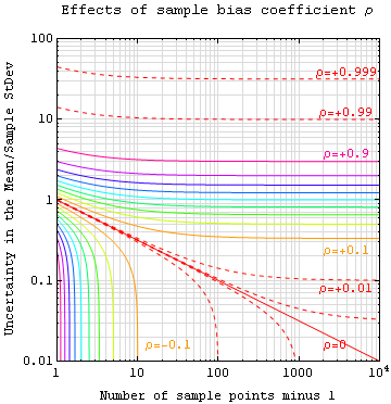
Note: Sample StDev above is Sqrt[SampleVariance/N].
The more difficult question is this: What sample bias coefficient should I expect? In general, one can only determine this by detailed measurements on a specimen with statistical properties like the specimen from which the sample was drawn. If such measurements are possible, that's wonderful since coming up with an estimate for the specimen's autocorrelation as a function of lag, and then averaging over all point pairs in a given sample, is a straightforward process.
On the other hand, if you know a bit about how the specimen was put together then a correlation coefficient model might be able to help out. For instance, in the case of diffusion-limited precipitation say of oxygen in silicon, one expects a zone around each oxygen precipitate that is depleted in oxygen. Hence one might expect some anti-correlation to occur over distances larger than a precipitate. Another model is that of randomly mixed grains. This may be reasonable for some rocks, and certainly for meteorites formed by random compaction of accreting material. Let's take this last model a bit further.
If your specimen is a random conglomerate of homogeneous grains, one can estimate the sample bias by first estimating the "containment probability". This is the probability that points located a distance L from a randomly chosen point will be in the same "grain" as that first point, and hence correlated in composition. Containment probabilities are also useful when estimating the effect of finite path-length radiation from one grain on another, for example in modeling the cathodoluminesence age of a rock.
A plot of this probability for various grain shapes in one, two and three dimensions is shown below. Note that the value for a cube is only approximate since we've not come up with an analytical expression for it yet.

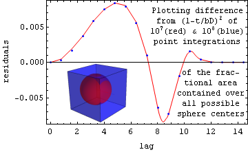
However a fairly simple approximation for containment probability, namely (1-t/(bD))2 for t<bD where t is lag, D is side, and b is the cube root of 30/4π, is quite good for the cube case as shown below. For the case when D=8, the lines in the plot show the difference between a Monte Carlo integration of the exact theory and this simple model. The blue points were obtained by averaging 100 million randomly-chosen lags, while points along the red line gave similar values using only 10 million each. As you can see, there are systematic errors in the analytic approximation, but their magnitude is always less than 0.01.
A convolution of the containment probability with itself, for the case of cubic grains of side d in a cubic sample volume of side D, yields the correlation coefficient described in the abstract:
 .
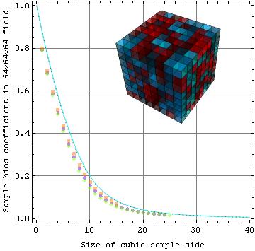
.The plot below compares model points (red dots) to a numerical integration of the exact theory calculation (cyan line). The results also compare favorably to several random experimental samplings of a cubic specimen (shown) of 83=512 cubes each 8 distance units (voxels) on a side. Hence there are 86 or about a quarter of a million voxels in the specimen to "sample".
Below we compare the same sample bias coefficient model (red curve) to experimental analyses of two dimensional specimens of various types. The ripple specimen (shown) has a phase-randomized ring of chosen frequency in their Fourier transform. The binary ripple specimen has further gone through binary segementation into two levels before analysis.

* These properties of sample bias coefficient were first outlined in this Appendix from my Ph.D. thesis. /pf