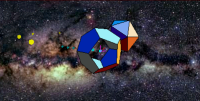
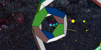
Check out the interactive model below by moving the mouse over its window. The force on the primary orbiter is plotted as a red line, the orbiter's velocity is in yellow, and the magnetic field at the orbiter is plotted in magneta. The force law used is Lorentz's qv×B, with dipole* and loop axis** fields sewn together with an azimuthal wire field falling off as one over distance-from-wire***. (Suggestions for improvement there are invited.) Objects shadowing the primary orbiter are three and six iterative time-steps back. A series of yellow dots, at 12 step intervals, is also left behind in its path.
* the dipole vector field a distance r, from the center of
a radius R loop, is
B~μoIR2{3(x/r)(z/r),3(y/r)(z/r),3(z/r)2-1}/(4r3).
** axis field for a radius R loop is z-ward with
Bz~μoI/(2(R2+z2)3/2).
*** magnitude goes as
Bwire~μoI/(2πrdist).
Time passes in the simulator when the mouse is over the window. The mouse can be used to re-orient the view (Drag), and to zoom in (Shift/DragDown). Javascript buttons below let you choose a few different orbits, and text boxes/buttons below that let you load and read out orbiter coordinates. Double-clicking on the model stops the simulation, and allows you to "drag" the primary orbiter to other orbits as well. The present version of the simulator uses full-increment integration. Half-increment and Runge-Kutta versions are in the works. Puzzler #1: With respect to the initial viewing direction, is the current in the loop going clockwise or counterclockwise?
The Load/Read coordinate buttons and windows above allow more quantitative experimentation, e.g. by letting you type in your own initial position and velocity coordinates. Thus you might search for initial conditions that... (i) result in surprising or even chaotic trajectories, (ii) highlight limitations of the numerical integration techniques currently in use, or (iii) illustrate intellectually interesting physcial phenomena.
What other trajectory explorers do you think might be interesting? For example, how about a three-body problem simulator, or far-time and traveler-time views of orbital and/or rain frame trajectories around a black hole? Would the trajectory of an electron in an energy-filtered microscope, or an ion in a mass spec, be fun to explore? How about trajectories in a spinning space station with artificial gravity? Even better, how about a traversable wormhole in your living room?
Notes on classroom use: These web accessible tools, like other empirical observation simulators here, are designed not to take up class time but to be explored by students elsewhere, e.g. as part of a take-home test or an external reporting project that might later be subject to classmate peer review.
Acknowledgement is due particularly to
Martin Kraus
for his robust
Live3D
applet.
The galactic panorama is copyright Axel Mellinger, and is adapted
here with permission, from his
300MB
All-Sky Milky-Way. Thanks also to former grad student researcher
Noom Pongkrapan for the
simulator border. Although there are many
contributors, the person responsible for errors is P. Fraundorf. This
site is hosted by the Department of Physics and Astronomy at UM-StL.
MindQuilts
site page requests ~2000/day approaching a million per year. Requests for
a "stat-counter linked subset of pages" since 4/7/2005:
.