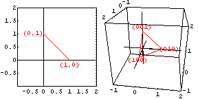
If you have N numbers that are positive and add up to one, then all possible values of those numbers plot within a finite N-1 dimensional figure. That's because the locus of such points in N-dimensional space is the N-1 dimensional analog of a triangle (i.e. an N-1 simplex)! For example, the composition of a binary solid-solution series can be represented by a straight line (1-simplex) that runs from (1,0) to (0,1). The composition of a ternary mixture in 3-space falls within a flat 2D triangle (2-simplex) with vertices at (1,0,0), (0,1,0) and (0,0,1). The figure at right illustrates how each of these structures is embedded in the higher dimensional space of which it is a part. The 3D locus in four-dimensional space of a quaternary mixture is, similarly, a tetrahedron (3-simplex) with vertices at (1,0,0,0), (0,1,0,0), (0,0,1,0), and (0,0,0,1). Higher dimensional spaces work the same way, although they (and their embeddings) are harder to visualize. Probabilities as well as compositions are generally positive numbers that, taken together in a complete set, all sum to 1. Thus N probabilities can also be mapped to the space within an N-1 simplex.
The red wire-tetrahedron below encloses the space of possible values for any four mutually-exclusive probabilities p11, p12, p21, and p22. The indices on these probabilities are meant to be more specific: pij is the joint probability that subsystem A is in state i, and subsystem B is in state j. We're thus focusing on the special case in which there are two subsystems (A and B), each of which can be in one of two states (like tossed coins, or half-integral spins). Marginal probabilities are the probabilities that one system is in the first or second state, regardless of what the state of the other system is. In the plot below, for example, Ap1 = p11+p12 represents the marginal probability that system A is in its state number 1, while Bp1 = p11+p21 is the probability that system B is in its state number 1.
The curved surface in the tetrahedron is the locus of probability assignments for which subsystem A and B states are not correlated with one another. This is true when pij = Api*Bpj for i,j=1,2. This surface is parameterized (criss-crossed) with lines of constant marginal probability. If one imagines similar surfaces moving outward toward both points of maximum mutual information, this structure can also be used to represent the "fitness landscape" for a simple two-layer, two state-per-layer, system evolving so as to maximize its correlation with the outside world.
The green line represents that direction along which mutual information is used to measure deviations from uncorrelated, for a given set of marginal probabilities. The mutual information between the two systems is zero on the uncorrelated surface. The point on that surface, projected from a system point in the direction of the green line (constant marginal probability), serves as the "net surprisal reference"" for the system's mutual information measurement. The blue dots are separated by 0.1 bit of mutual information, so that the two subsystems can show at most (as the green line reaches one of the red ones) one bit of mutual information.
For example, two ordinary pennies would be likely to have equal probabilities of state A (heads) or state B (tails). Moreover, they would normally have uncorrelated values. Their joint probabilities would therefore all be 1/4, and they would plot where the uncorrelated surface intersects the green line. If someone "weighted" one of the two coins, the probability of tossing heads with it might no longer be 1/2, so that the two-subsystem point might move along the uncorrelated surface toward one of the uncorrelated sheet edges. On the other hand, if someone were instead to glue the two unweighted pennies head-to-tail with one another, then the system would continue to plot on the green line but its point would move up to one of the intersecting red lines because the previously separate coin states would now be correlated i.e. if one penny was "heads-up" the other would be heads as well. Another physical model that this applies to is a set of two (correlated or uncorrelated) binary spins.
Not sure, but we're thinking about adding a pair of half-bit mutual-information iso-surfaces to the model above, and about a separate 4-state system model (like that below) showing constant thermodynamic net-surprisal iso-surfaces with respect to the center point at (1/4,1/4,1/4,1/4). A 2x2 array of such tetrahedra would allow us to treat the case of 3 coupled spins, where even more interesting collective effects begin to emerge*, rather than the two coupled spins examined above. Even the tetrahedron with corners p111=1, p211=1, p222=1 and p121=1 should make an interesting comparison to the model above, since most types of 1-faces (edges) and 2-faces (tetrahedron facets) of the spin triplet's 5-simplex (which all-told has 15 edges and 20 triangular facets) are illustrated. We might also further increase model interactivity (if there's interest) by providing compositional and probability versions to which you can add your own data points and axis labels...
Here's a version of the tetrahedron above, with the 0.3 bit net surprisal contour calculated with respect to the central position {1/6, 1/6, 1/6, 1/6, 1/6, 1/6} for a 6-probability 5-simplex projected into 3 dimensions. This is also the 0.3 bit contour relative to {1/6, 1/6, 1/6, 3/6} in the N=4 3-simplex as well.
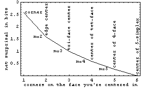
In the original 5-simplex, net surprisals with respect to that central position remain finite as one moves out to the corners, as shown below. Net suprisals of one corner with respect to another, however, do not.
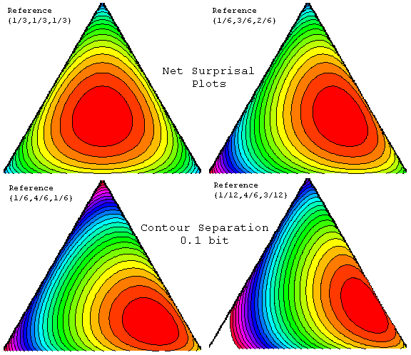
Projecting into 2D onto an equilateral triangle (a 3-vertex 2-simplex), one can profile these net surprisals quantitatively. Here the contours are spaced by 0.1 bit of net surprisal with respect to the reference or expected. As the expected value moves away from the center point, note that net surprisal at the "far points" goes up. In addition to the N=3 probability distribution illustrated directly, these values of net surprisal also apply to projections from higher dimension, as long as probability is equally partitioned over the probabilities summed over in the process. Thus with respect to {1/6, 1/6, 1/6, 1/6, 1/6, 1/6}, the upper left plot also contours net surprisal for {f1+f2, f3+f4, f5+f6}, the upper right plot for {f1, f2+f3+f4, f5+f6}, and the lower left plot for {f1, f2+f3+f4+f5, f6}. Projections of the lower right plot from the N=6 5-simplex require an off-center reference, like {1/12, 1/6, 1/6, 1/6, 1/6, 3/12}.
To illustrate the utility of these plots for more than three probabilities, the animation below examines what happens to these contours for the uniform reference, when one moves from N=6 to N=5 independent probabilities.
